Learning can be defined and understood as the processes that
allow animals to detect systematic relations among events in their world.
For example, events are often correlated because of the causal relations among
them. Thunder consistently follows lightning and the expectation of
hearing thunder that occurs when one sees a flash of lightning is an example of
classical conditioning - the well-studied and ubiquitous learning process that
allows animals to detect systematic relations among the occurrence of two
(or more) kinds of events. Another very well-studied kind of systematic
relation among events is the fact that particular behaviors are reliably
followed by particular events, usually because the behavior is the cause of the
event. For example, a rat for whom food is programmed to reliably follow
the pressing of a lever in a Skinner Box soon learns to press the lever.
This learning about the systematic relation between one's own behavior and its
outcomes, of course, is instrumental conditioning. These forms of
associative learning have been described as the means by which the nervous
system detects systematic patterns in the relations among event occurrences
(e.g., Dickinson, 1980).
But relations among the occurrence of events is not the only
sort of relations among events that exist. At least three other kinds of
relations among events have been shown to support learning (Table 1). If there is a sequential relationship among events presented in
a series, animals come to be controlled by that relationship. For example,
if a rat is presented with a series of trials in which the number of pellets
provided as reinforcement systematically increases (or decreases) over the trial
series, running speed systematically increases (or decreases) over the trial
series (e.g., Capaldi, Blitzer, & Molina, 1979; Hulse & Dorsky, 1980). It
has been argued that this control is produced by a learning process that
represents the sequential relationship among the events, in this case by representing the
systematic increase (or decrease) in reward magnitude (Hulse, 1978).
Learning processes that are sensitive to temporal relations
among events have received a great deal of experimental and theoretical
attention. The study of animals exposed to events that are systematically
separated in time by intervals on the order of seconds to minutes has led to
well developed theories of learning systems specialized for learning about the
temporal relations among events (see Church, 2002 for a review).
|
Table 1: Proposed Relational Learning Processes |
|
Learning Process |
Type of Relation |
Example |
|
Classical Conditioning |
Correlation Among Event Occurrences |
One event (e.g., bell) consistently followed by a second
event (e.g., food)
|
|
Instrumental Conditioning |
Correlation Between Behavior and Event |
Behavior (e.g., lever press) consistently followed by
event (e.g., food pellet) |
|
Serial Learning |
Ordered Change in Event Property |
Increase in Reinforcement Magnitude Over Trials |
|
Interval Timing |
Systematic Temporal Interval Between Events |
Reinforcement Available on a Fixed Interval Schedule |
|
Spatial Pattern Learning |
Systematic Spatial Relations Among Events |
Reinforcement Arranged in a Consistent Spatial Pattern |
This cyber-chapter is about the means and mechanisms by which
spatial
relations are learned. The focus is on a series of
experiments that attempt to isolate learning about the spatial relations among
locations and the control of behavior by those relations.
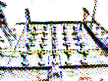
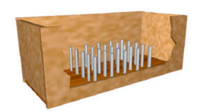
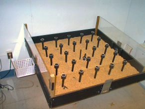
Two illustrations of the Pole Box apparatus used in our spatial pattern
learning experiments are shown below (Figure 1A, 1B). Poles are equally
spaced, with separations in different versions of the apparatus ranging from 12
cm to 21 cm. The poles are arranged in a matrix - we have used apparatus
with 4 X 4, 5 X 5, and 4 X 5 matrixes of poles. There is a well on
top of each pole, in which a pellet (or other small food item) can be hidden.
In the critical conditions of our experiments, the location of the baited poles
varies unpredictably from trial to trial. Nevertheless, the baited poles form a
consistent spatial pattern over trials. Figure 1C shows one exemplar of each of three spatial
patterns for which we have evidence of behavioral control and, by inference, of
spatial pattern learning. Spatial pattern learning can be contrasted
with other forms of spatial learning that have been described, as outlined in Part II:
Varieties of Spatial Learning of this cyberchapter. The evidence for
control by the square (top panel), line (middle panel), and checkerboard (bottom
panel) patterns is reviewed in Part III:
Spatial Pattern Learning in the Pole Box.
"Of all the constraints on nature, the most far reaching are
imposed by space. For space itself
has a structure that influences the shape of every existing thing."
(Stevens, 1974) |
Tolman's (1948) original
construct of a cognitive map regained
influence with the publication of O'keefe and Nadel's (1978) The Hippocampus
as a Cognitive Map. O'keefe and Nadel argued that the hippocampus is
the site of spatial representations and that information stored by the
hippocampus includes the spatial relations among locations in familiar
environments. Publication of this work marked the beginning of a
wave of experimental and theoretical work aimed at understanding the
physiological and cognitive mechanisms of spatial learning and memory.
 |
Figure 2A.
Beacon homing. Animal moves toward (or away from) a perceived,
localized cue.
|
 |
Figure 2B. Piloting. Animal moves toward (or away from)
a location defined by its spatial relations to perceived,
localized cue(s).
|
 |
Figure 2C.
Control by geometry. Animal moves with reference to the
perceived shape of a space (or a perceived cue that is determined by
the shape of the space (see Cheng,
this volume).
|
 |
Figure 2D.
Dead Reckoning. Animal moves according to internal cues that
are determined by the direction and distance of its recent movement
(e.g., vestibular cues).
|
Several mechanisms have since been identified that allow animals
to navigate accurately in two-dimensional and three-dimensional space. A relatively simple mechanism is often referred to as beacon
homing (Gallistel, 1990). A beacon is a perceived landmark (visual,
auditory, or chemical cue). Beacon homing is simply moving toward a beacon
(Figure 2A). Of course, moving toward a beacon is not a trivial problem -
there must be some means of determining when one is moving toward the beacon.
An increase in the apparent size of the perceived beacon, for example, has been
identified as a mechanism by which some animals used visual stimuli as beacons.
Detecting an increase in the concentration of a chemical is a cue that can be used to detect the source of
a chemical through beacon homing; it is used by many animals to find food.
Beacon homing allows animals to locate a place, as long as there
is a perceivable cue coincident with the goal location. When cues are
present, but not coincident with the goal location, many animals are able to
pilot to a goal location using landmarks that have a consistent spatial relation
to the goal location and to each other (Gallistel, 1990). In order to do so, the
animal must have learned the spatial relations among the landmarks and goal location(s)
(Figure 2B). Such learned spatial relations correspond closely to the
cognitive mapping process that Tolman described.
Cheng (1986) first proposed that a global spatial frame, within
which the goal location(s) is consistently located, can serve as learned spatial
cues. The evidence for this view is described by
Cheng and Newcombe
elsewhere in this book. The evidence indicates that animals acquire a
representation of the spatial properties of the global space in which they
search for food (e.g., a rectangular arena). The representation includes
the location of the goal(s) within that spatial framework. The location of
a food site or other important place is coded in terms of its spatial relation
position within the represented spatial frame. Cheng argued that this process
constitutes a geometric module which functions somewhat independently of
other forms of spatial control. In Figure 2C, an animal is
navigating with a rectangular area (represented by the orange rectangle
surrounding the shark). A cognitive representation of the geometric
properties of the area is represented by the orange rectangle inside the
animal.
Beacon homing, landmark use, and control by geometry all rely on
the presence of perceived visual (or auditory or chemical) cues. In
contrast, the spatial pattern learning that is the subject of the present
chapter occurs in the absence of perceivable cues. Rather, the context of
the spatial pattern learning that we have studied is the configuration of hidden
food locations. No beacons or landmarks correspond to the correct food
locations. In our experiments, rats are foraging in a rectangular
arena, similar to the ones used by Cheng (1986). However, the food
locations on any particular trial are not predictable in terms of location
within the arena. Thus, beacons, landmarks and geometric cues can not be
involved in the ability of rats to find the baited poles in the pole box task.
Another mechanism known to be involved in animal navigation is
dead reckoning (also known as path integration). Internal
movement cues (provided primarily by the vestibular system) allow the animal to
integrate its position in space relative to a starting point (Biegler, 2000;
Collett, Collett, Bisch, & Wehner, 1998; Etienne, Berlie, Georgakopoulos, &
Maurer, 1998; Mittelstaedt & Mittelstaedt, 1980; Wehner & Srinivasan,
1981). Thus,
when an animal moves a given distance and direction (indicated by the arrow
behind the animal, Figure 2D), the vestibular system provides information about the
distance and direction moved (relative to a starting location). There is
abundant evidence that this information allows the animal to find its way back
to the starting location. It has been argued (e.g., Gallistel, 1991) that
this ability is mediated by a representation that has the form of a vector
coding the distance and direction to the starting location (indicated by the
arrow in the animal's head below). This vector is continuously updated as
the animal moves. In the pole box task, the baited locations have consistent
spatial relations with each other. Thus, it is possible that dead
reckoning could be involved in the mechanism by which those relations are
learned.
|
|
Figure 3A.
The pattern exemplar changes unpredictably from trial to trial. (Animation
will show a sequence of examples)
|
|
|
Figure 3B. Video example of pole box trial.
|
Brown and Terrinoni (1996)
reported the first evidence for control by a spatial pattern of baited poles.
In a 4 X 4 pole box, one of nine possible 2 X 2 square arrangements of four
baited poles was available on each daily trial. Figure 3A illustrates the critical fact that,
over trials, the identity of the baited poles was unpredictable prior to each
trial, but the baited poles were consistently arranged in the square pattern.
The video to the right (Figure 3B) shows a typical trial in the 4 X 4 pole box apparatus,
after some exposure to a square pattern. The baited poles during this
sample trial are indicated by the red rings (superimposed on the video for
illustration purposes).
As this sample trial suggests, rats come to be controlled to some extent by the
consistent spatial arrangement of the baited poles. Prior to each, the
location of the baited poles is unpredictable unless, of course, the rats can
perceptually detect them - using odor cues, for example. We have
consistently found in all of our pole box experiment that, in fact, the rats are
no more likely to choose a baited pole than would be expected on the basis of
chance. Thus, the rats are not locating the baited poles using odor
or any other perceptual cues.
If a rat learned that the baited poles are arranged in a 2 X 2 square
pattern, then the discovery of one or more baited poles might be expected to
provide information about the location of the remaining baited poles.
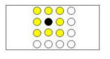
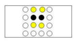
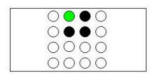
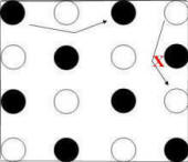
In particular, after the discovery of one baited pole (indicated by the black
circle in Figure 3C, left panel), the square pattern indicates that the remaining
three baited poles must be among the eight nearby poles (indicated by the yellow
circles).
After the discovery of two adjacent baited poles (Figure 3C, center panel), the
square pattern indicates that the remaining two baited poles must be one of two
adjacent pairs of poles (indicated by the yellow circles). And after three
baited poles have been discovered (Figure 3C, right panel), the the location of
the one remaining baited pole is completely determined.
 |
Figure 4.
Logic of the Brown and Terrinoni analysis of choice conformity to
the square pattern following discovery of a second baited pole. 1
= first baited pole chosen during trial; 2 = second baited pole
chosen during a trial; S = poles adjacent to the second baited pole
chosen that conform to the square pattern; X = poles adjacent to the
second baited pole that do not conform to the square pattern.
Green arrows show conforming moves and red arrows show
non-conforming moves. The analysis compares the proportion of
moves conforming to the pattern to the proportion expected on the
basis of chance, based on these values for each rat cumulated over
trials.
|
 |
Figure 5.
The proportion of choices following discovery of a second baited
pole that conformed to the square pattern was greater than the
proportion expected on the basis of chance. The difference
between empirical and expected performance increased over trial
blocks.
|
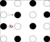
The clearest evidence for behavioral control by the square
pattern comes from an analysis of the choices that immediately follow the
discovery of the second and third baited poles. Following the second
discovery of the baited pole (marked "2" in Figure 4), is the rat
relatively more likely to next choose a pole that conforms to the pattern (i.e.,
the two poles marked "S")? An accurate assessment of
such control by the pattern requires that two other factors affecting pole
choices be considered. First, there is a strong tendency to choose poles
that are spatially proximal to the most recently chosen pole. Thus, the
analysis compares choice of poles that conform to the pattern ("S" poles in the
figure) to choice of poles that are also adjacent to the most recent choice but
do not conform to the pattern (the "X" pole in the figure). Also, rats may
have a tendency to avoid revisits to poles chosen earlier in the trial, just as
they avoid revisits to maze arms in a radial-arm maze (Olton & Samuelson, 1976).
In fact, it is clear that rats are able to avoid pole revisits in the pole box
task, albeit to a much lesser extent than they avoid revisits of maze arms in the
radial-arm maze. To control for any possible confounding of control by the
pattern with control by previous pole visits, only initial visits to poles are
included in the analysis (i.e., revisits of poles are not included in the
analysis).
Figure 5 shows the results of this analysis in the
experiment reported by Brown and Terrinoni (1996) in which rats were exposed to
a square pattern for 120 daily trials. The empirical results, shown
in blue, are in terms of the proportion of choices made immediately
following the discovery of a second baited pole and to a previously unvisited
and spatially adjacent pole which were to a pole consistent with the square
pattern (i.e., choices to poles represented by the "S" poles in Figure
4). These data can be compared to the proportion that would be
expected on the basis of chance, shown in red. This proportion is
given by the proportion of previously unvisited and spatially adjacent poles
that were consistent with the pattern.
So, in the example trial above, the Proportion Expected is:
2 ("S" poles) / 3 ("S" poles + "X" poles, assuming that none of them have been
previously visited during the trial) = .67
Note that the expected proportion is affected by the number of adjacent poles
that have been previously visited during the trial and by the location of the
square exemplar on any given trial (i.e., whether the square is in the center,
edge, or corner of the pole box matrix). The proportions obtained and
expected were calculated for each rat during each trial block. The rats
chose poles that were consistent with the square pattern more often than
expected by chance, and this difference increased over the three trial blocks.
Choices following the third discovery of a baited pole were
analyzed separately in a directly analogous manner. Figure 6 shows
an example of the possibilities for choices included in the analysis following
discovery of the third baited pole. In this case, there is always exactly
one pole consistent with the pattern (i.e., the remaining baited pole) and up to
two choices that would be inconsistent with the pattern.
|
 |
Figure 6. Logic of the Brown and Terrinoni (1996) analysis of choice conformity to
the square pattern following discovery of a third baited pole. 1
= first baited pole chosen during trial; 2 = second baited pole
chosen during a trial; 3 = third baited pole chosen during a trials;
S = poles adjacent to the third baited pole chosen that conform to
the square pattern; X = poles adjacent to the third baited pole that
do not conform to the square pattern. Green arrows show
conforming moves and red arrows show non-conforming moves. The
analysis compares the proportion of moves conforming to the pattern
to the proportion expected on the basis of chance, based on these
values for each rat cumulated over trials.
|
 |
Figure 7.
The proportion of choices following discovery of a third baited pole
that conformed to the square pattern was greater than the proportion
expected on the basis of chance. The difference between
empirical and expected performance increased over trial blocks.
|
The obtained and expected proportions of choices made that were
consistent with the pattern in Brown and Terrinoni's experiment are shown in
Figure 7.
Again, rats chose poles consistent with the square pattern more often than
would be expected on the basis of chance and the tendency to do so increased
over the course of the experiment.
We have replicated Brown and Terrinoni's evidence that choices
come to be controlled by a square pattern of baited poles several times (Brown,
Yang, & DiGian, 2002; DiGian, 2002; Lebowitz & Brown, 1999; Wintersteen,
2003).
One important detail in all of these experiments is that we use
several methodological and analytic techniques to be sure that the choice of baited
poles can not be explained by any perceivable cue. The most obvious
possibility is that the rats can use odor to locate baited poles. In
all of our recent experiments, we use poles that include a "sham" bait pellet.
The structure of these poles is shown in Figure 8.
|
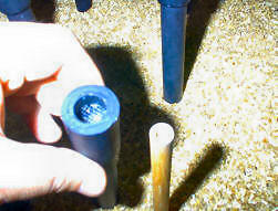 |
Figure 8. Outer sleeve of pole (being held) and inner core (to right).
Sham pellet (on every pole) is placed in well at top of inner core.
Baited poles have a second (accessible) pellet in the well at top of
sleeve.
|
Each pole
is constructed with an inner core of dowel. A single "sham" pellet is
hidden in a well drilled in the top of the pole. The core is covered by a
sleeve made of PVC (removed from the core for purposes of this illustration).
The top of the sleeve includes a well in which a single pellet can be hidden
when the pole is baited. The floor of the well is nylon mesh material.
Thus, any odor from the 45 mg sucrose pellets is present in every pole.
However, only the baited poles contain a pellet that is accessible to the rat.
The second means of determining whether odor or any other other perceptual cues
play a role in locating the baited poles is to examine rats' ability to locate
the first baited pole discovered during each trial. Because the location
of the baited poles varies unpredictably from trial to trial, the ability to
locate the baited poles should be no more accurate than expected on the basis of
chance - unless the rats can detect the pellets perceptually.
We have
examined this aspect of performance in each of the experiments we have done
using the pole box apparatus. We have not found any evidence that rats
locate the first baited pole any better than would be expected on the basis of
chance. (See Lebowitz & Brown (1999) for a discussion of some of the complexities
involved in this measure.) Thus, the ability of rats to locate additional baited poles
after discovering the location of one baited pole must be based on learning the
pattern.
|
|
Figure 9. Several exemplars of the row pattern. (Animation will show a sequence
of examples)
|
In several experiments, we have shown that choices can also be
controlled by a linear pattern of baited poles. In some of these
experiments, the baited poles form either one row or one column of the
pole matrix (Brown & Terrinoni, 1996; Brown, DiGello, Milewski, Wilson, & Kozak,
2000). In others, the baited poles form a linear pattern with the same
orientation on every trial, but a different row of the matrix (DiGello, Brown, &
Affuso, 2002; DiGian, 2002). This latter version of a linear pattern is
illustrated in Figure 9.
The video in Figure 10 shows a trial in the experiment of DiGello, et
al. (2002). One of the four rows of poles
is baited on each trial. The baited poles on this sample trial are
the four poles in the row adjacent to the wall of the pole box that cuts across
the lower right corner of video (indicated by the green arrows superimposed on
the video). Those four poles are baited on 25%
of the trials, with each of the three parallel rows of poles also being baited on 25%
of the trials.
|
|
Figure 10. Video of trial in experiment using the row pattern.
The poles baited on this example trial are indicated by the
green arrows. |
 |
Figure 11.
Explanation for control by a square pattern in terms of overlap
of spatial generalization gradients around the previously
discovered poles. In the this case the gradients produced
by two baited poles discovered earlier in the trial overlap at
the location of poles that conform to the square pattern, but
not at the location of poles that do not.
|
Two features of the linear
pattern are particularly interesting
for our understanding of pattern learning. First, an alternative
explanation for control by the square pattern involves spatial gradients of
generalized excitation surrounding baited poles that have been discovered.
That is, when a rat finds a baited pole, perhaps the area surrounding the pole
increases in attractiveness - a form of generalization.
Figure 11
illustrates how two overlapping gradients of excitation (represented by the
green areas) centered on two
previously discovered baited poles can result in more generalized excitation to
poles that are consistent with the square pattern (i.e., the poles above and
below the previously discovered baited poles) than to adjacent poles not
consistent with the pattern (i.e., the pole to the right of the 2nd discovered
pole). Thus, control by the square pattern could be explained by
generalization. A line pattern, however, requires that rats make choices that
are inconsistent with generalization. Thus, control by the line pattern rules out a general explanation of control by spatial patterns in terms of
generalization.
The second important feature of the the row pattern is
the fact that locating an unbaited pole (as well as locating a baited pole)
provides potential information - if one pole in a row is not baited, then none
of the poles in that row are baited. We have
shown that rats' choices are controlled by this contingency (DiGello et al., 2002).
DiGello, et al. tested rats in a 4 X 4 pole box in
which one of four columns of poles was baited on each trial, as in the
video in Figure 10. If a rat has discovered one or more baited poles (e.g., the pole
indicated in black in Figure 12A), then the remaining baited poles are determined - they
are the other poles in the same column (e.g., the poles indicated in yellow).
If a rat chooses a pole and that pole is not baited (e.g., the pole
indicated in green in Figure 12B), then none of the remaining three poles in that column
are baited, and the baited poles are in one of the three remaining columns.
Thus, although determining that a pole is not baited does not provide as much
information as discovering a baited pole, it does narrow down the possibilities. DiGello, et al. (2002) showed that rats come to be controlled by both sources of
information. They acquire both a tendency to choose poles in the same
column after choosing a baited pole and a tendency to choose poles in a
different column after choosing an unbaited pole.
|
 |
 |
Figure 12.
(A)
Positive information provided by choice of a baited pole when a
column pattern is in force. When a baited pole is chosen
(black circle), the remaining baited poles (yellow) are in the same
column. (B)
Negative information provided by discovery of an unbaited pole when
a column pattern is in force. When an unbaited pole is chosen
(green circle), the remaining poles in that column are not baited
(unfilled circles) and the baited poles are in one of the three
other columns (yellow, orange, or red).
|
|
|
Figure 13. Animation of the two exemplars of a checkerboard pattern.
|
 |
Figure 15. Results from Brown, Zeiler, & John
(2001). By Trial Block 3, Adjacent moves were more
likely following choices of an unbaited pole, whereas
Skip and Diagonal moves were more likely following
choice of a baited pole. These results provide
evidence of control by the checkerboard spatial pattern.
|
A third spatial pattern that we have studied is the
checkerboard pattern. This pattern has only two exemplars, as illustrated in
Figure 13.
Our analysis of control by the checkerboard pattern
involves consideration of the relative probability of three kinds of "moves"
(transitions from one choice to the next). The first is choice of a pole
adjacent to the pole most recently chosen. In Figure 14, filled circles represent
baited poles and the arrows indicate two examples of an adjacent move (left
panel). An
"adjacent" move is consistent with the checkerboard pattern following choice of
an unbaited pole (i.e., an adjacent move following choice of an unbaited pole
would result in choice of a baited pole). However, an adjacent move
following choice of a baited pole would result in choice of an unbaited pole.
 |
 |
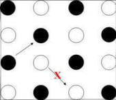 |
Figure 14. Transitions from one choice to the next
that are diagnostic of control by the checkerboard pattern. Black
circles represent poles that were baited at the beginning of the
trial. Arrows show diagnostic transitions. Arrow
with red "X" indicates transition
contra-indicated by pattern.
Left Panel: Adjacent moves correspond to choice of a
baited pole only if they are made from an unbaited pole.
Middle Panel: Skip moves correspond to choice of a baited pole
only if they are made from a baited pole.
Right Panel:
Diagonal moves correspond to choice of a baited pole only if
they are made from a baited pole.
|
A "skip" move is choice of
a pole separated by one pole
(in either a row or column of the pole matrix) from the most recently chosen
pole. As shown in Figure 14 (middle panel), a skip move is consistent with the checkerboard pattern (i.e., would
result in choice of a baited pole) following choice of a baited pole, but not
following choice of an unbaited pole.
Finally, a "diagonal" move is choice of a pole that is
adjacent along a diagonal axis to the most recently chosen pole. As shown
in Figure 14 (right
panel), a diagonal
move (like a skip move) is consistent with the checkerboard pattern following
choice of a baited pole, but not following choice of an unbaited pole.
Brown, Zeiler, & John (2001) found that rats acquire a tendency
to make adjacent moves following choice of an unbaited pole and skip and diagonal
moves following choice of a baited pole. Figure 15 shows their data
in an experiment with 60 daily trials. Over the course of three blocks of
20 trials each, the relative likelihood of adjacent moves increases following
choice of an unbaited pole and decreases following choice of a baited pole.
The opposite chance occurs for skip moves and diagonal moves. Thus, rats
acquire tendencies to make choices that conform to the checkerboard pattern in
which baited poles are arranged. This evidence for control by a
checkerboard pattern was replicated by Brown and Wintersteen (2004).
These results show that rats can learn a
variety of spatial patterns. It should again be
emphasized that these are not spatial relations among particular
places defined by their location in allocentric
space. The location of food varies unpredictably from trial to trial.
Thus, the spatial relations among the baited locations must be abstracted from
any allocentric map that is anchored by specific locations in space. We
infer that an abstract representation of the spatial pattern is formed as the
rat experiences the spatial relations that exist among places where food has
been found within each trial. The next section
explores some mechanisms that might be involved in this ability.
|
|
|
Figure 16. (A) An S-R explanation of correct responding
following discovery of two baited poles when pole are
baited in a square pattern. (B)
An S-R explanation of correct responding following discovery of two baited poles
when poles are baited in a linear pattern.
|
Clearly, spatial choices can be controlled by the
spatial relations among goal locations despite the fact that those goal
locations are not designated by any visual or other perceivable beacons,
landmarks, or geometric cues. What is the mechanism of this spatial
pattern learning?
One possibility is that rats acquire response tendencies that
result in choice of poles with particular spatial relations to previously chosen
poles, and that such acquired response tendencies constitute the mechanism of
control by spatial patterns (Olthof, Sutton, Slumskie, D'Addetta, & Roberts,
1999). After being exposed to the square pattern, for example, a rat
might acquire the following response tendency: After finding two adjacent
baited poles, turn left or right and choose the next pole (Figure 16A). This rule
would result in finding a third baited pole. It requires that the rat
discriminate and remember the spatial relation between the first two baited
poles and then respond in a manner that is contingent on that relationship.
A similar (although somewhat more complex) rule could be
acquired that would increase the likelihood of choosing the fourth baited pole
in a square pattern. The response rule that would produce control by a linear pattern
is the converse of the one that would be acquired for a square pattern: After
finding two adjacent baited poles, move in the same orientation as those two
poles and choose the next pole (Figure 16B).
In the case of a checkerboard pattern, the description of a
response tendency explanation of control by the pattern corresponds directly to
the measure of control by the checkerboard pattern described in
Part III: Spatial
Pattern Learning in the Pole Box.
That is, rats develop a tendency to make adjacent moves following choice of an unbaited pole and/or a tendency to make skip & diagonal moves following choice
of a baited pole.
Brown, Zeiler, and John (2001) showed that the acquisition of
such response tendencies cannot explain control by spatial patterns, at least in
the case of the checkerboard pattern. Brown, et al. (Experiment 2) exposed
rats to a checkerboard pattern in a 5 X 5 pole box. Barriers (constructed
of plastic mesh material allowing the rats to see through the barriers)
prevented moves to poles in the same row or column (Figure 17). Thus, without walking
around a barrier, rats could only choose poles along a diagonal axis.
 |
Figure 17. Exemplars of the checkerboard pattern, with clear plexiglass walls forming diagonal alleys of poles shown.
This arrangement was used during the training phase of
Brown, Zeiler, and John's (2001) experiment. |
Therefore, during this training phase, a rat could not
have acquired response tendencies that correspond to adjacent or
skip moves. Nevertheless, when the barriers were removed, the
rats immediately demonstrated a stronger tendency to make adjacent
moves following choice of an unbaited pole
and a stronger tendency to make skip moves following choice of a baited pole.
This result shows that spatial relations among goal locations control behavior
in the absence of specific response tendencies.
If the mechanism of control by spatial patterns is not the
development of response tendencies, then what is it? We conclude that an
abstract representation of the spatial relations among the goal locations is
acquired. Such a representation would allow novel paths from one goal
location to another to be followed. The logic of the Brown, Zeiler, and
John's (2001) experiment and the conclusion that a flexible spatial representation
is necessary to explain the results are analogous to Tolman, Richie, and
Kalish's (1946) classic "shortcut" experiment and the resulting argument that a
flexible representation (cognitive map) of familiar locations is acquired.
However, there is a critical difference between the spatial relations involved
in the pole box task and the spatial relations among particular locations. In the case of Tolman's experiment, as in
the case of almost all more recent and current work on cognitive mapping, the locations are specific
locations in allocentric space, defined by spatial cues (e.g., beacons,
landmarks, geometric cues). In the pole box task, however, the goal
locations vary unpredictably from trial to trial. The goal locations,
therefore, must be coded in a temporary manner. The relationships
among the baited locations, on the other hand, are consistent across trials and
must be coded in a permanent manner in order to effectively control choices in
accord with the pattern. This is the sense in which the spatial pattern
must be abstract: it must be abstracted from the relation of the particular locations that are
baited on particular trials.
In order to abstract the spatial relations among goal locations,
given that the goal locations change unpredictably in allocentric space, rats
must somehow be perceiving the spatial relations among the baited poles found
during individual trials. Two possible mechanisms for doing so can be
distinguished. First, a working memory system could be used to code
the allocentric location of poles previously discovered during a trial.
The spatial relations among those locations could then be determined on the
basis of working memories for their locations. The abstracted spatial
relations among baited locations would then be coded in a more permanent memory
system. According to this view, the process of spatial pattern learning is
analogous to concept learning in that the spatial relations are abstracted from
particular exemplars of baited pole locations experienced over trials.
|
|
Figure 18. Video of rat in in polebox with feedback stimuli indicating
chosen
arms.
Click image to play video.
|
Alternatively, a dead reckoning system could be used that
integrates the distance and direction from each baited pole discovered to the
next. According to this view, rats need not code the locations of
particular baited poles during the trial. Instead, their spatial
relationship is coded directly in terms of the vector provided by dead reckoning
as the rat moves in the pole box and chooses poles. A new vector is
initiated each time the rat discovers a baited pole. The resulting set of
vectors specifying the relations among each pair of poles forming the pattern
constitutes the learned spatial pattern.
We recently completed a series of experiments designed to
investigate the possibility that working memory for the location of previously
discovered baited poles is involved in pattern learning. To do so, we
developed pole box apparatus that allowed us to provide visual cues
corresponding to poles visited during each trial.
The video in Figure 18 shows a trial from an experiment using the first
of two versions of this apparatus.
As the rat visits poles, a spotlight (produced from above using a data
projector) marks the location of visited poles. It was expected that such
cues would allow the rats to make fewer revisits of poles. The question
was whether it would also enhance control by the checkerboard pattern of baited
poles. If so, that would constitute evidence that working memory is also
used to keep track of where the previously discovered baited poles were, and
that these temporary memories about the elements of particular exemplars of the
pattern are involved in the ability to learn the abstracted pattern.
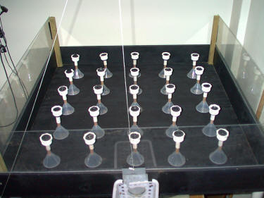 Figure 19. (A) Apparatus used by Brown and Wintersteen. Translucent base of each pole can be illuminated
from below
Figure 19. (A) Apparatus used by Brown and Wintersteen. Translucent base of each pole can be illuminated
from below
|
|
 |
(B)
Close-up of poles in the Brown and Winterseetn apparatus. Pole
in foreground is not illuminated. Two poles in background are
illuminated. Pole illumination was used as a cue indicating
whether pole had been visited earlier during the trial.
|
|
Unfortunately, the visual cues had no effect on either pole
revisits or control by the pattern. It is likely that this failure of the
cues to affect behavior was due to the brightness of the light produced by the
data projector. We suspect the the rats may not have been able to
discriminate the cues because they were masked by the ambient light produced by
the projector.
A modification of the technique used to provide visual cues
resulted in cues that did affect behavior. The base of the poles in this
second version of the apparatus (shown in Figure 19A) were constructed of translucent
material and mounted on top of holes cut in the floor of the arena. A data
projector was used to project light up from underneath the apparatus, thereby
allowing poles to be individually illuminated (as shown in Figure 19B).
Brown and Wintersteen (2004) trained rats with one of the two
exemplars of the checkerboard pattern defining the location of the baited poles
on each trial. During training, the base of the pole was illuminated
whenever a rat choose the pole (or, for half of the rats, all the poles were
illuminated at the beginning of the trial and the illumination was turned off
when the rat visited a pole). During a test phase, half of the
trials did not involve use of the visual cues (the illumination of the poles did
not change). This allowed comparisons of performance with and without the
visual cues corresponding to visited locations. The visual cues did
enhance the ability of the rats to avoid revisits to poles visited earlier
during the trial. However, there was no evidence that the cues had an
effect on control by checkerboard spatial pattern. Because visual cues
corresponding to visited poles facilitated the ability of rats to avoid revisits
of those poles but had no effect on control by the checkerboard pattern, Brown
and Wintersteen argued, the working memories for pole locations used to avoid
revisits must not be involved in the acquisition of pattern learning or in the
use of learned patterns to locate baited poles. They suggested that two
separate working memory systems may be used in the pole box task: one set of
working memories reduce visits to those (previously visited) locations and a
second set of working memories code the location of previously discovered baited
poles.
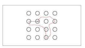 |
Figure 20.
Illustration of path integrated spatial relation between two poles.
Rat follows path indicated in red from on pole to the other, but
codes the spatial relation between them as indicated by the arrow,
based on information provided by path integration.
|
Although the existence of two separate working memory systems can explain the
dissociation of memory for previous pole visits from control by spatial
patterns, another possibility is that working memory for the location of
previously visited poles is not involved in the learning or use of spatial
patterns at all. Instead, rats
could acquire the spatial pattern of baited poles using dead reckoning. Dead
reckoning could be used to detect and code the spatial relations among the poles
baited in a pattern if discovery of a baited pole defines the end of integration
of one dead reckoned vector and the beginning of another. Furthermore, the
product (vectors) of the dead reckoning process would have to be stored across
trials. Biegler (2000) has proposed an analogous function of dead
reckoning in the development of allocentric cognitive maps (see Biegler,
this volume).
Figure 20 shows a hypothetical path of a rat as it moves
from one baited pole to another. Note that the route of the rat might be
quite indirect and might include visits to other (non-baited) poles. The
suggestion is, however, that the discovery of a baited pole defines the end of
an instance of path integration (and the beginning of a new one). Thus,
each transition from one baited pole to another produces a vector (the arrow in
Figure 20) that defines the spatial relationship between
those two baited poles. Each transition from one baited pole to the next
would produce one such vector.
 |
Figure 21. Hypothetical vectors representing abstracted spatial
relations
among locations (green dots). These could be formed as a result of
moving among the locations via dead reckoned spatial relations.
|
The resulting vectors would be cumulated over discoveries of baited poles both
within a trial and over trials. Over the course of trials, the square,
line, and checkerboard patterns would result in a set of vectors that code the
spatial relationships among the baited poles in the three patterns.
In Figure 21, the vectors produced by dead reckoning are represented by
the lines connecting the (green) goal locations. The goal locations are
defined exclusively in terms of the vectors. That is, there is no coding
of the location of the goal locations in allocentric space. Their position
is learned only in relation to each other. Dead reckoning provides a
mechanism for this relational spatial coding.
 |
Figure 22. Hypothetical vectors representing
abstracted spatial relations
among two kinds of locations - baited (green dots) and unbaited (red dots)
|
A weakness of this account of spatial pattern learning is that it does not
explain the ability of rats to choose in accordance with the pattern after
choosing an unbaited pole. This ability was clearly shown in the
case of a line (row) pattern by DiGello, et al. (2002). Furthermore, the
tendency to choose adjacent poles following choice of an unbaited pole in the
checkerboard pattern also indicates that rats not only learn the spatial
relationships among baited poles, but also learn the spatial relationships
between baited poles and unbaited poles.
It is, of course, possible to extrapolate
the dead reckoning view of pattern learning by proposing that the
spatial relationship between all pairs of consecutively chosen poles
is discriminated using dead reckoning and that the bait status of the poles is also
coded along with the resulting set of vectors. An illustration of one
version of this idea is shown below for the checkerboard pattern (Figure 22). The
green nodes represent baited poles and the red nodes represent the unbaited
poles that separate the baited poles in the rows and columns of the matrix.
Learned vectors define the relations among the baited locations and between the
adjacent baited and unbaited locations.
Thus, dead reckoning provides a potential mechanism for abstracting the spatial
relations that control choices in the pole box. We do not yet have any
direct evidence for or against the possibility that dead reckoning is providing
this information. Abstraction of the spatial relations among baited
poles may be mediated either by working memories for the particular locations
baited on individual trials or by dead reckoning.
Brown, M.F., DiGello, E., Milewski, M., Wilson, M., & Kozak, M.
(2000). Spatial pattern learning in rats: Conditional control by two
patterns. Animal Learning & Behavior, 28, 278-287.
Brown, M.F., & Huggins, C.K. (1993). Maze-arm length affects a
choice criterion in the radial-arm maze. Animal Learning &
Behavior, 21, 68-72.
Brown, M.F., & Lesniak-Karpiak, K.B. (1993). Choice criterion
effects in the radial-arm maze: Maze-arm incline and brightness.
Learning and Motivation, 24, 23-39.
Brown, M.F., & Terrinoni, M. (1996). Control of choice by the
spatial configuration of goals. Journal of Experimental
Psychology: Animal Behavior Processes, 22, 438-446.
Brown, M.F., & Wintersteen, J. (2004). Spatial pattern learning and
spatial working memory. Learning & Behavior, 34, 391-400.
Brown, M.F., Yang, S.Y., & DiGian, K.A. (2002). No evidence for
overshadowing or facilitation of spatial pattern learning by visual
cues. Animal Learning & Behavior, 30, 363-375.
Brown, M.F., Zeiler, C., & John, A. (2001). Spatial pattern learning
in rats: Control by an iterative pattern. Journal of Experimental
Psychology: Animal Behavior Processes, 27, 407-416.
Cheng, K. (1986). A purely geometric module in
the rat's spatial representation. Cognition, 23,
149-178.
Dahl, D., & Winson, J. (1985). Action of
norepinephrine in the dentate gyrus. I. Stimulation of locus
coeruleus. Experimental Brain Research, 59, 491-496.
Dallal, N.L., & Meck, W.H. (1990). Hierarchical
structures: Chunking by food type facilitates spatial memory.
Journal of Experimental Psychology: Animal Behavior Processes, 16,
69-84.
Dickinson, A. (1980). Contemporary animal
learning theory. Cambridge: Cambridge University Press.
DiGello, E., Brown, M.F., & Affuso, J. (2002).
Negative information: Both presence and absence of spatial pattern
elements guide rats' spatial choices. Psychonomic Bulletin &
Review, 9, 706-713.
Gallistel, C.R. (1990a). The organization of
learning. Cambridge, MA: M.I.T. Press.
Kamil, A.C., & Jones, J.E. (2000). Geometric rule
learning by Clark's nutcrackers (Nucifraga columbiana). Journal
of Experimental Psychology: Animal Behavior Processes, 26,
439-453.
Lebowitz, B.K., & Brown, M.F. (1999). Sex differences in spatial
search and pattern learning in the rat. Psychobiology, 27,
364-371.
O'Keefe, J., & Nadel, L. (1978). The
hippocampus as a cognitive map. Oxford: Oxford University Press.
Olthof, A., Sutton, J.E., Slumskie, S. V., D'Addetta, J., & Roberts,
W.A. (1999). In search of the cognitive map: Can rats learn an
abstract pattern of rewarded arms on the radial maze? Journal of
Experimental Psychology: Animal Behavior Processes, 25, 352-362.
Olton, D.S., & Samuelson, R.J. (1976). Journal of Experimental
Psychology: Animal Behavior Processes, 2, 97-116.
Pearce, J.M., Ward-Robinson, J., Good, M., Fussell, C., & Aydin, A.
(2001). Influence of a beacon on spatial learning based on the shape
of the test environment. Journal of Experimental Psychology:
Animal Behavior Processes, 27, 329-344.
Stevens, P.S. (1974). Patterns in nature. New York: Little,
Brown & Co.
Suzuki, S., Augerinos, G., & Black, A.H. (1980). Stimulus control of
spatial behavior on the eight-arm radial maze. Learning and
Motivation, 11, 1-18.
Thinus-Blanc, C. (1996). Animal spatial cogntion: Behavioral and
neural approaches. Singapore: World Scientific.
Tolman, E. C. (1948). Cognitive maps in rats and men.
Psychological Review, 55, 189-208.
Acknowledgements
The work
reviewed in this chapter was supported by grant IBN-9982244
from the National Science Foundation. I thank the many
graduate and undergraduate students who have contributed to this
project. |

©2006 All copyrights for the individual chapters are retained by the
authors. All other material in this book is copyrighted by the editor,
unless noted otherwise. If there has been an error with regards to
unacknowledged copyrighted material, please contact the editor
immediately so that this can be corrected. Permissions for using
material in this book should be sent to the editor.