Entire Set of Printable Figures For

The Perception of Similarity - Blough

Click here for pdf version

Figure 1.   People differ in their perception of hue similarity.  Most people see a yellow square at left and a reddish circle at right; they see the dots comprising each form as dissimilar in hue from the surrounding dots.   Persons with a form of colorblindness known as "protanopia" or "red-green blindness" will probably see the yellow square but not the circle;  for them, the dots in the circle are similar in hue to those in the background.

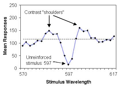
Figure 3.  An example of the dimensional contrast effect.  Wavelengths appeared on a response key for 20 sec in random sequence, and responding was rewarded on 10% of these trials.  In addition, 597 nm appeared without reward on half of the trials.  Contrast appears as "shoulders" near the negative stimulus.  (Data from D. Blough, 1975).

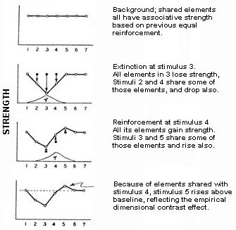
Figure 4. A common-elements account of the dimensional contrast effect (redrawn from D. Blough, 1983).

Note on Metric Axioms

In the geometric approach, dissimilarities are treated as distances in space, and they must follow the rules that govern metric distance between objects.  Specifically, the dissimilarity  function d assigns to every pair of objects A and B a nonnegative number according to the following three axioms:

•  Minimality:   d(A,B) >= d(A,A) =0;  The dissimilarity  between two objects is greater than or equal to the dissimilarity between an object and itself, which is zero.
   
• Symmetry:   d(A,B) = d(B,A);  Dissimilarity is not directional; the dissimilarity of A to B is the same as the dissimilarity of B to A.
  
• The triangle inequality:   d(A,B)  +  d(B,C) >= d(A,C); A and C cannot be farther apart in similarity space than the sum of their distances to any other object B

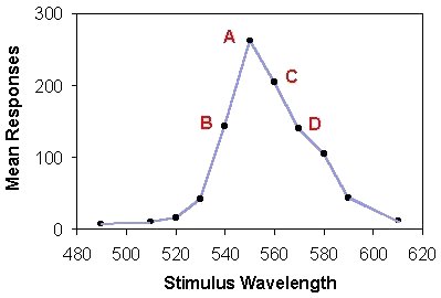
Figure 8.  This is one of the first pigeon generalization gradients ever determined (redrawn from Guttman & Kalish, 1956). Prior to the test the birds were reinforced for pecking at a stimulus patch of 550 nm. The test responses to that wavelength are at A.  What can be said about the similarities among stimuli at A, B, C, and D, and others?

Figure 9.   How overlapping gradients can be used to find a unique similarity scale for the stimulus continuum (here, wavelength).  At top, two empirical gradients have rather different shapes when plotted against wavelength.  At bottom, the wavelength scale has been altered until the gradients are as nearly the same as possible.  Shepard (1965) used five overlapping gradients to define the new similarity scale.

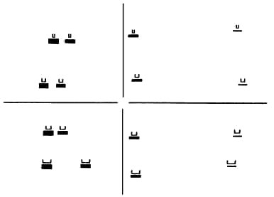
Figure 12. This is a two-dimensional Euclidean plot of the similarities derived from odd-item search reaction times.  Distances between any two items represent their dissimilarities.  The scaling algorithm found two psychological dimensions corresponding to the physical differences in U width (vertical) and block size (horizontal). (Based on D. Blough, 1988).

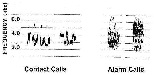
Figure 19. The frequency spectra of two samples of budgerigar contact calls and two of alarm calls. (Figures redrawn from Dooling et al, 1990).

Figure 20. A MDS and cluster analysis of budgerigar contact calls and alarm calls.
 (Figures redrawn from Dooling et al, 1990).