Functional Considerations in Animal Navigation:
How do you use what you know?
Robert
Biegler
Norwegian University of Science and Technology
|
Abstract This chapter is an attempt to analyse animals’ navigation strategies by starting with the most basic problem "How can I get to a specific place X?," attempting to find a simple solution, considering the limitations, and deriving from those additional requirements that a navigation strategy may usefully meet. Going through several iterations of this process leads to six major conclusions: One, the nature of the readout mechanism is as important as the kind of representation and the rules for storing information in it. Two, navigation is possible without representing spatial relationships. Three, there is a whole spectrum of navigational systems, which do not fall into two distinct classes of simple associative models and complex mapping models. Four, readout mechanisms are often domain-specific and species-specific. Five, the short cuts and instantaneous transfer often considered critical tests of cognitive mapping are computationally rather simple at the level of readout. Six, path integration is sufficient to solve a wide range of ecologically relevant navigation problems, namely those that involve determining an animal’s own location relative to familiar other points. |
I. Computational Goals of and Requirements for Navigation
In the most general terms, the goal of navigation is to have the capacity to reach a specific location different from the current one. In other words, the question is not "where is X?," but "how can I reach X?". This destination X could be food, water, shelter, cover from predators, or some other resource. The most basic requirement for this is to recognise a goal location once it has been reached. Recognition of a location once there will be taken for granted from here on, ignoring that there could be interesting complexities to this process (T. S. Collett, pers. comm.). If an animal were capable only of this recognition, a destination could only be reached through a random walk. This may never lead to the goal, or may lead to the goal only after a very long time. Such limitations suggest further functional requirements, for example, that a path to a goal should be efficient. This progressive development of functional requirements orders models of navigation in terms of what they can do, regardless of the details of their internal processes. This emphasis on functional considerations highlights the importance of how information is read from a representation and that navigation does not necessarily require the representation of spatial parameters such as angles and distances. To avoid excessive length, the discussion of navigation models is quite selective, rather than comprehensive. In particular, I will focus primarily on landmark-based navigation strategies and mention only the most important aspects of navigation based on path integration, which has been discussed in detail elsewhere (Biegler, 2000; Collett & Collett, 2000; Etienne & Jeffery, 2004; McNaughton et al., 1996; Mittelstaedt, 2000)
II. Some Models of Navigation
2.1. Trail Following
A very simple way of returning to a place is to lay down a trail on a solid substrate when leaving and to retrace it later. This may be called the Hänsel and Gretel or the Ariadne strategy. The information stored in memory could be an association between the destination and the substance used to make the trail. Retrieval of that association would identify the appropriate trail. However, a performance rule or readout mechanism is needed to use that information to reach a goal. In the case of a chemical trail, an animal with a receptor both to the right and left has a simple algorithm for following the trail: if the concentration of the trail substance differs at the two receptors, turn towards the side where the concentration is higher. Other algorithms are possible.
Limpets can follow their own slime trails to return to the spot on the rock where the shell exactly fits the surface and will provide a secure seal (Blackford-Cook, 1969; Cook, Bamford, Freeman, & Teidemann, 1969). Other molluscs use the same strategy (Cook, 1977). Ants lay odour trails to recruit other foragers (Wilson, 1971). Large enough animals using a specific path often enough will trample a trail, which then may aid navigation. It is not clear, though, that any species relies exclusively on trail following for navigation.
The use of self-generated trails does not require representation of spatial relations in any form. The only information that needs to be stored and retrieved is an association between the destination and the trail. However, without performance rules or readout mechanisms, the information stored in associations would be useless. It is the spatial distribution of the trail substance or physical disturbance in combination with the algorithm used to determine which way to turn that take the animal to its destination. Learning and retrieval can follow general rules of associative learning, but the information is then used in task-specific computations.
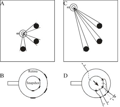
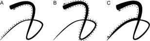
Figure 1. A) An animal that lays down a trail of a marker substance from home to a destination can follow this trail again, later, with minimal computational effort, but is largely bound to the original path, however inefficient. If the animal can detect small enough variations in the strength of the odour trace (symbolised here by the width of the trace), it is possible to cut out loops by choosing, at an intersection, the branch of the trail with the strongest odour. However, this decision rule works only when following the odour trail in the original direction. B) When trying to retrace the path, the same decision rule would lead back to the starting point. C) If either the same or another individual has followed the trace in the original outward direction, as in A), and laid another odour trail on top, it becomes possible to follow the trace in both directions by following the strongest trace. In any case, there is no way of choosing between goals on the basis of distance, or of other short cutting besides removing loops.
Trail following is computationally simple, but has several limitations. Because the mere presence of a trail provides no spatial information, the animal cannot choose the closer of two otherwise equivalent destinations. To be identifiable, each destination needs its own recognisable trail. Marker substances also tend to fade with time. Until they do fade, they could be followed by competitors or predators which may either use and deplete the resource or eat the animal that laid down the trail (Clifford et al.,, 2003; Gehlbach, Watkins, & Kroll, 1971; Gonor, 1967; Paine, 1963; Webb & Shine, 1992). In addition, a trail may lead along a quite tortuous path. If the trail crosses over itself, so long as the animal is travelling in the same direction as when it laid down the trail, a simple rule can cut out the loop and get the animal to its destination: follow the strongest concentration (Figure 1A). However, if the animal is travelling in the other direction, the stronger branch of the trail will be the one leading into the loop. When the animal then returns to the crossing point a second time, the stronger branch will be the one leading the animal back where it just came from (Figure 1B). In a social species, a second individual following the trail and laying down another trail on top would cut out the loop and ensure that the branch leading back would be the strongest at an intersection (Figure 1C). Social caterpillars do follow the strongest trail at an intersection (Fitzgerald, 2003), while ants use the bifurcation angle at branching points of the trail network: the average bifurcation angle when outbound is 50 - 60°, so both branches should require a small turning angle, while when inbound one branch should require a large turning angle (Jackson, Holcombe, & Ratnieks, 2004). I am not aware of any data indicating how solitary animals solve this problem. Possibly the simplest solution is to avoid it by not looping back over a trail when first laying it down, which could be achieved by restricting headings to a 180° range. Two further possibilities are assessment of the age of a trail independent of strength, for example, by assessing the ratio of trail components that have different decay rates (the predatory snail Euglandina rosea can determine the polarity of conspecifics’ trails, though the mechanism by which it does so is not known; Clifford et al., 2003), or by using a trail following algorithm more complex than following the strongest concentration. Thus, even a navigation strategy as apparently primitive as trail following may contain some complexities.
The functional limitations suggest additional properties which would make a navigational system more useful. It should be able to identify and find one among several possible destinations. The path there should be reasonably efficient. Relevant information should only be identifiable as such in memory, rather than recognisable by other organisms.
2.2. Beacon Navigation
If a destination has a conspicuous feature perceptible at a distance, an animal only needs to recognise and approach this beacon. The information stored in memory would be an association between beacon and destination. There is a distinction between what information is stored and how it is used. In this case, navigation would consist of keeping the beacon at a fixed angle relative to the direction of locomotion, usually straight ahead. Biased detours (Collett, Dillmann, Giger, & Wehner, 1992) involve using beacons only for very rough course corrections. Following an extended cue, for example, a river's edge, is another special case of beacon navigation. These methods of navigation have been called 'guidance strategies' by O'Keefe and Nadel (1978).
Direct approach to a perceptible beacon assures an efficient path. If a beacon at a destination is too far to be seen from the starting point of a journey, following a sequence of beacons may still lead to the goal. This could be described as chains of stimulus-stimulus associations (Deutsch, 1960). Reaching a beacon puts the animal in a position to pick up and approach the next beacon in the chain. Short cuts become possible if a beacon known to be farther on in the sequence becomes visible early, perhaps after removal of an obstacle. Identification of beacons allows choice between different destinations.
There are limitations. Knowing only a sequence of beacons, it is impossible to tell how long a path would be either in absolute terms or compared to an alternative. A specific chain of beacons may define only a one-way route. For example, when hiking along a forest trail it is easy to turn left on reaching a stream and walk until reaching a cottage. When returning, it may be much more difficult to find the same trail. Likewise, a bee may easily see a hill covered with flowers, but the hive could be rather less conspicuous at the same distance. There may not even be any useful beacon at a destination. Such limitations are no reason to avoid the use of beacons entirely. Bees and wasps commonly deviate from direct routes towards a feeding station, heading towards conspicuous landmarks first (Chittka & Kunze, 1995; Collett, 1995; Collett & Baron, 1994; Von Frisch, 1967). The limitations of beacons suggest that their use should be combined with that of other navigational strategies, the way bees do (Cheng, 2000).
III. Use of Snapshots
Figure 2. The snapshot model of Cartwright and Collett (1982). (A) The bee learns a snapshot at the goal. Landmarks are black discs. (B) The inner circle is the snapshot, the outer circle the current view on the retina. The bee's orientation, marked by a tail, remains constant. (C) Approach to the goal. (D) The bee matches areas on the snapshot with the closest areas on the retina that have the same colour. It flies towards areas that are smaller than remembered (in this case landmarks and the two gaps between them) and away from areas larger than remembered (the region without landmarks behind the bee). This is shown by radial unit vectors. If an area is farther right than remembered, the bee flies to the right, as shown by tangential vectors. The flight direction results from addition of all these unit vectors. The length of unit vectors does not vary with the size of mismatch. Adapted from Cartwright and Collett (1983).
If there is no beacon, the next option is to store a "snapshot" or "local view" of the environment as seen from the goal. (As use of these terms is quite inconsistent, it must be made clear that here they refer to image-like representations without information about distances of objects or the spatial relations between them, other than their retinal sizes and their separation on the image.) There are at least five ways of using a snapshot for navigation.
3.1. Image Matching
Cartwright and Collett (1982, 1983) proposed an algorithm, intended to describe visual navigation in honey bees, which effectively creates a virtual beacon. When at a destination, the bee is assumed to store in memory a two-dimensional image of the scene visible there. When navigating back to that place, the bee retrieves this snapshot and compares it with the scene it sees at its current location. The two variables that the algorithm attempts to match in snapshot and scene are the orientation and angular extent of landmarks and of the empty spaces between them. The retinal image and retinal snapshot are modelled as dark areas (landmarks) and light areas (empty spaces) on a circle (Figure 2). The middle of each area on the snapshot is determined and paired with the middle of the nearest corresponding area on the retinal image. The algorithm then combines tangential movement vectors (to bring matched areas into alignment) with radial movement vectors (to match the angular extent of areas) to produce an overall flight vector. The lengths of the tangential and radial vectors are not related to the magnitudes of the discrepancies. There is no quantitative measure of mismatch. The flight vector does not represent distance and direction to the goal. It merely points in a direction that takes the bee closer to the goal. Like conventional beacons, the combination of snapshot and algorithm has a "catchment area" within which the features stored in the snapshot are perceptible and the discrepancy between snapshot and scene is small enough to allow a match. Within this catchment area, in principle the image matching algorithm should lead the animal to the goal regardless of whether the area traversed is familiar or not. However, the snapshot must be kept in the correct compass orientation, requiring either a mental rotation, or alignment of the body. Bees do the latter (Collett & Baron, 1994), so the effective catchment area is not centered on the snapshot, but displaced to one side.
Image matching accounts well for bees' behaviour when pinpointing a goal and their reaction to landmark displacements (Cartwright & Collett, 1983; review in Collett, 1996). Although it was originally suggested that the virtual beacons provided by image matching might be used over much the same distances as actual beacons, in practice bees use image matching only during the last portion of their trajectory to a goal (reviewed by Cheng, 2000).
3.2. Gradient Descent by Minimisation of Visual Mismatch: Biased Random Walk and Taxis
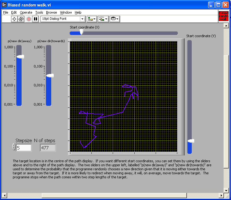
Figure 3. Simulation of two biased random walks from a home location to a destination, under the assumption that mismatch is proportional to distance from the destination.
The image in the figure is a link to the simulation program. Click on the image to download or open the simulation program - in most operating system environments, you should be able to "open" the file to run the simulation without downloading it to your computer. However, you will probably FIRST have to download the LabView Runtime engine on your computer - and then INSTALL it - before being able to run this or the other simulations in this chapter.
If an animal can compute a quantitative measure of mismatch between a remembered snapshot and currently perceived scene, it can move so as to reduce that discrepancy. A quantitative measure of mismatch effectively creates a gradient. Biased random walk and taxis are two simple procedures for gradient descent. To generate a biased random walk, check the rate of change of discrepancy when moving and choose a new direction randomly at a rate related to the rate of change of discrepancy. If discrepancy decreases quickly, keep going for some time; if it increases slowly or even decreases, pick a new direction very quickly (see Figure 3 for a simulation).
To use taxis, an animal must make the connection between turning right or left and an increase or decrease in the rate of change of discrepancy. Then the animal can turn towards the destination until the increase in concentration is fastest. Benhamou and Bovet (1992) described statistical measures for distinguishing these two strategies. Whether either taxis or biased random walks are ever used by computing mismatch with reference to visual landmarks is uncertain. Buresova, Homuta, Krekule, and Bures (1988) tested for the use of taxis by comparing the paths of rats in the watermaze (Morris, 1981) in two conditions. One was a standard training situation with lights on so that the rats could use visual cues. In the other condition, the lights were off and distance from the goal was signaled by the pitch of a tone. In darkness, the shape of the path corresponded to that typical of a taxis mechanism, but not when the lights were on and the rats could use visual landmarks.
3.3. Mismatch Comparison: How to Pick the Best of Possible Next Steps
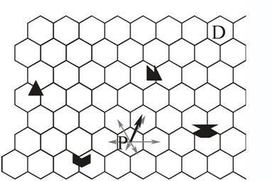
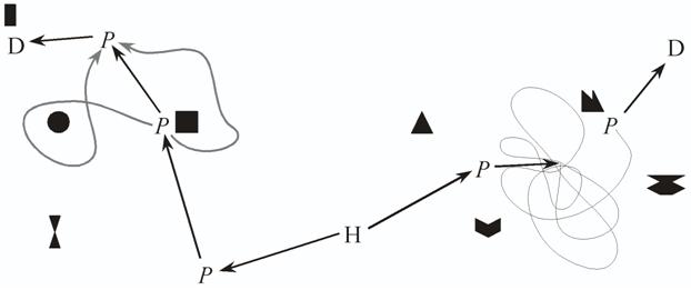
A very different way of navigating is possible if the animal stores in long term memory not only the snapshot taken at the destination, but also snapshots in a large number of other places. The animal does not compare the current view with the snapshot taken at the destination. The current view only serves as a retrieval cue for snapshots taken at all the places adjacent to the animal's current location. The animal then compares the discrepancies between the snapshot taken at the destination and each of those it has retrieved from memory (Benhamou, Poucet, & Bovet, 1995). From the adjacent places it could then choose the one with the smallest discrepancy. Benhamou et al. found that performance of a computer model is more robust if it adds up all vectors to adjacent places, weighting them according to their discrepancies with the destination (Figure 4).
Figure 4. Navigation by comparing mismatches. Each hexagon stands for a place where a snapshot has been taken. At a place P the animal retrieves from memory the snapshots taken at adjacent places and computes their mismatches with the snapshot taken at the destination. The vectors to each adjacent place (grey arrows) are then weighted according to the corresponding mismatches. The weighting is shown here by the different lengths of vectors. The sum of these weighted vectors (black arrow) gives an estimate of the best next step and of the direction of the destination. Depending on the measure of mismatch, the differences between mismatches of opposite locations may give a good estimate of the distance of the destination.
The particular measure of mismatch used by Benhamou et al. allows an estimation of the distance of a goal from the bearings and vertical angular sizes of landmarks. No other distance cues (e.g., motion parallax, looming, accommodation, or binocular divergence) are used. All spatial information is computed from the comparison of snapshots. The animal's memory does not store spatial relations between places or responses linked to places. Because this strategy depends on retrieving snapshots from adjacent places, mismatch minimisation is only possible in areas the animal is familiar with. Keith and McVety's (1988) experiment, indicating that rats can benefit from being placed at the goal without knowing snapshots at a release site and places on the way to the goal, would suggest that mismatch comparison either is not the navigational strategy used in this case, or that it is not the only one.
3.4. Stimulus-Response Associations
A snapshot may be used only to recognize or identify a place, ignoring any measure of mismatch. Place recognition would not, by itself, give an animal any information on where some other place of interest might be. Navigation would proceed by associating each place with a specific response. Normally a sequence of responses would be necessary, as the animal travels through a number of places on the route to its destination. If the animal keeps track of the response it makes in each place, it can, on arrival at its destination, reinforce a whole sequence of responses. It could give most weight to the most recent responses, as those are most likely to have contributed to actually reaching the destination.
This way of learning is path-specific. Only those responses made on the way to the destination can be reinforced. Any other experience of traveling through the same places, either during exploration or on the way to different destinations, has no influence on learning to find the current goal. In contrast to the mismatch comparison model of the last section, there is no latent learning.
The response may either involve traveling for a specific distance or until reaching the next place that is recognised as a 'ballistic' response. One important characteristic of such a ballistic response is that, by itself, it lacks any method of error correction, or even of detecting when an error has occurred. If a deviation from the correct course led an animal past the place it aims for, it would just keep going, and would not even know when it has gone too far. Even if the deviation is small enough that the place aimed for is recognised, there is no way either to adjust the response for the deviation, or to get to the centre of that snapshot, so that the next response is actually appropriate. There are two ways around this problem. One is to store in memory so many snapshots and their associated responses that any error will lead to a familiar place, even if not the one aimed for. A critical feature of this navigational strategy is its path-dependence. Using ballistic S-R associations, an animal can only reinforce the responses it made on its way to a goal, and it can only have one response in each place. One consequence is that while learning to find one destination, any other experience travelling through the same area, on the way to other destinations or during exploration, is irrelevant (see Figure 5). Rats are definitely not that dependent on specific experience (Chew, Sutherland, & Whishaw, 1989; Keith & McVety, 1988; Sutherland, Chew, Baker, & Linggard, 1987; Whishaw, 1991). However, Collett, Collett, Bisch, and Wehner (1998) reported that desert ants exiting from a runway would first turn in the accustomed compass direction and walk on that heading for some distance, before turning into the direction of the nest as specified by the global path integrator.
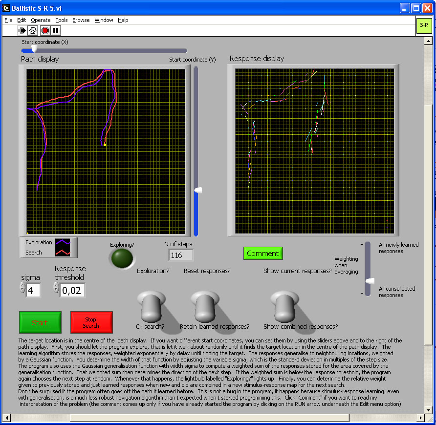
Figure 5. The image in the figure is a link to the simulation program. Click on the image to download or open the simulation program - in most operating system environments, you should be able to "open" the file to run the simulation without downloading it to your computer. However, you will probably FIRST have to download the LabView Runtime engine on your computer - and then INSTALL it - before being able to run this or the other simulations in this chapter.
In this simulation, during exploration the model animal starts off from the location you specify using the sliders, takes off in a random direction, then after each step alters direction randomly to the left or right by 10 degrees until either it comes near the goal in the centre of the display, or you stop it. During exploration, the program stores the direction of each step not only at the coordinate where a response was made, but also at neighboring coordinates, with response strength being a Gaussian function of distance. The width of that Gaussian generalization function can be set at either Xσ x step size or 2Xσ step size using the control labeled “sigma." The length of each step is 7, in a 501 x 501 grid of positions. The strengths of all stored responses decreases by 0.5% after each step, giving an exponential decay over time, thus giving greater weight to more recent responses. Random search can take a long time, and because the goal is arbitrary anyway, you may stop at any time, switch from exploration to search, and see how good these stimulus-response associations are at following a path and cutting out loops.
During search, the program looks for responses stored not only at the exact current coordinate, but also, again with Gaussian weighting, at neighboring coordinates. The response threshold determines how low the cumulative strength of responses can be before the model again switches to random exploration. If and when it does so, an indicator lights up.
I have not had time to explore the behavior of the model in detail, but expect the following: The wider the generalization is during learning, the wider will be the trail of responses that search can pick up, and the more efficient the model will be at progressively shortening paths whenever it is on the inside of a curved path. Learning during search can reinforce responses further and would make the model more resistant to noise (not incorporated because it would slow down computation too much), but when the generalization curve is wide enough for substantial overlap with previous responses, learning during search would tend to keep the model going in the same direction, effectively increasing inertia. That would make sharp turns more difficult, and thus make it harder to cut out loops. There is nothing in the S-R associations that would keep the model animal to the centre of the trail of responses. In fact, because the model moves at a tangent to the path and step size if finite, instead of infinitely small, the model inevitably spirals out of a curve. To prevent this would either require an assessment of the total strengths of stored responses and an algorithm that treats this strength like an odour trail, or else the model would need to compute the outcome of the next step, then travel in the direction stored for that next location. Then it would not be a pure stimulus response model any longer.
A second way of correcting errors is to add a distance component to the response. Distance would have to be determined through path integration, if the assumption is to be maintained that the only thing landmarks do is to act as a retrieval cue for a response. Navigation would be route-based in that the animal must travel from one familiar point to the next, even though path integration puts no constraint (other than those of accuracy) on the paths between these points. That would already increase flexibility. Further, if on arrival at the end of such a response vector an animal has no response associated with that place, it can trigger a search procedure (Figure 6), or use one of the mismatch minimization algorithms. Triggering such behavioral programs only after traveling for the appropriate distance would make it likely that the current view of the environment most closely resembled the snapshot of the next destination, rather than leading the animal back to where it just came from.
There is still a limitation common to all ways of navigating by stimulus-response associations: S-R associations do not contain any information regarding the outcome of the response. They are habits. Given the stimulus, the animal will have a predisposition towards a particular response. Whenever an animal navigating that way comes across any place on a familiar route, it would tend to follow that route, regardless of what is at the end of the path and whether the animal needs that.
One way around that problem is to use separate maps of S-R associations for each destination. Choice of a destination then "loads up" the corresponding map, and although the animal’s behaviour is rigidly determined from there on, at least it is appropriate to the goal. However, rats appear to display still more flexibility than that. S. F. Brown and Mellgren (1994) found that information about locations of destinations is available to rats when choices are made. Also, in any radial maze experiment where animals do not use a stereotyped sequence of choices they must have information about what to expect at a location. To decide whether or not to walk down an arm the animal should remember whether it has already retrieved the food there. It must judge the likely outcome of its response. In Rescorla's (1991) terms, this excludes a pure S-R model and requires at least an association of the stimulus with a response-outcome complex, S-(R-O) for short.
An extremely simple form of using S-(R-O) associations constitutes the third way of correcting navigational errors: retrieve together with the response the snapshot of the next destination and use again a mismatch minimization algorithm. Just retrieving the snapshot most similar to the current view would not be good enough, because quite often that would be the location just left behind. This way of introducing information regarding outcomes would not change the behavior of the system much. However, there are other possibilities.
3.5. Stimulus-(Response-Outcome) Associations
Figure 6. Stimulus-response associations with a distance component. Place recognition is the cue for retrieval of the direction and distance of the next path segment to be traveled. If path integration is used to reach the next intermediate goal the animal is not bound to one specific path (grey arrows on the left). If there is an error (right hand path) the next familiar place could be reached either by random search under the control of path integration, as shown here, or by combining the S-R mechanism with, for example, image matching.
One way of introducing outcomes is to use a separate map of S-R associations for each desired destination. As only one response can be associated with each individual place representation, the maps would have to be completely separate for each destination, imposing a large memory load.
A second way of introducing outcomes into the associations is to set up a system that, given a stimulus, retrieves not only a response, but also the place where this specific response leads. If the animal can only retrieve the next place, knowledge of the outcome of the response is only useful for error correction. On the other hand, if the animal can chain responses and outcomes, the behaviour of the system is transformed. If the animal can follow a chain of responses to their ultimate outcome, it can simulate a path to a destination. Then knowledge of these ultimate outcomes makes storage of several possible responses at one place useful, because the animals can assess the consequences of each choice. In order to find a path to a final destination, an animal would need to simulate first all the possible current responses, i.e., going to all the places adjacent to its current position. For all those places it must again simulate the next set of possible responses, until one of the predicted outcomes is the desired destination. Then the animal must select, from all the responses it considered, only those that lead to the goal. Muller, Stead, and Pach (1996) provide a clear description of the necessary conditions for such a path search to be feasible. Schölkopf and Mallot (1994) published a detailed analysis of a model of this type, including a readout mechanism. Steinhage and Schöner (1996) have developed a model (with a distance component to the responses) for implementation in a robot.
I will not describe these models in detail. What matters here is that the second way of introducing outcomes can transform even a ballistic S-R system into one that can have many of the properties demanded from a cognitive map. The outcome of a response is arrival at another identifiable place. The representation of space consists of a network of nodes. The nodes correspond to places in the real world and the connections between nodes to responses. It is possible to find novel paths through the real world, given a search algorithm that can find corresponding paths through the network to a desired destination. A system of this type is not bound to specific paths anymore, whether the responses are ballistic or include a distance component. The system would still be restricted to navigation in familiar areas, because the animal needs experience of travelling between places in order to connect up the corresponding nodes in the network. It does not matter how that experience is gained, whether in exploration, or while travelling to some destination. Once the links between nodes are established, they are available for navigation to any place represented in the network. If the represented places are evenly spaced, or if they are randomly spaced at a similarly high density, then real world distances along any arbitrary path will be closely correlated to the number of nodes traversed on the equivalent path in the representing network. Such a network of stimulus-(response-outcome) associations (Muller et al. called it a ‘cognitive graph’) can thus be the basis for flexible navigation, though only if there is a suitable path search algorithm that reads the information stored in the pattern of connections between nodes and turns it into a path.
3.6. Reading Out a Vector
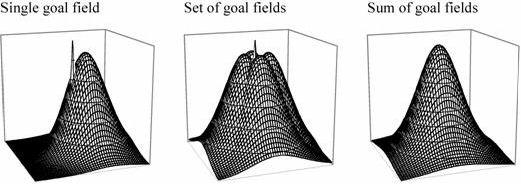
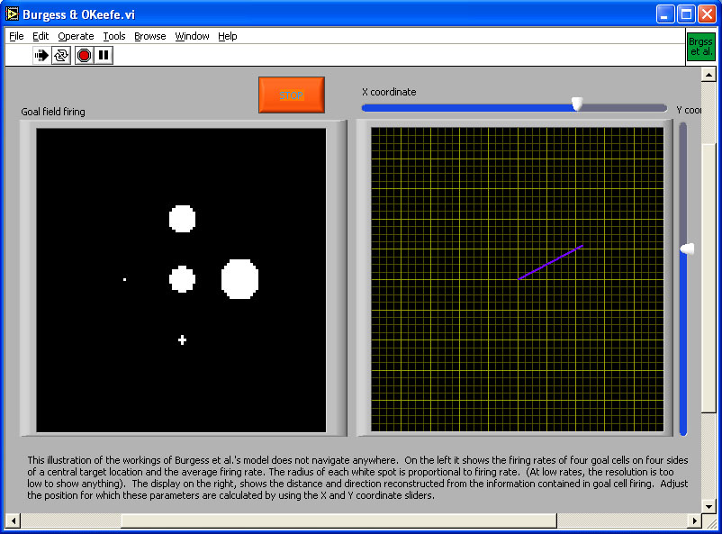
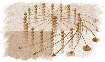
(A) (B) Figure 7. (A) Goal fields in Burgess et al.’s (1994) model. The spike in the left and centre diagram represents the goal location. A single goal field is offset from that location; the animal links the goal cell to place fields ahead of its current location by timing the strengthening of connections to the late phase of the theta cycle. If the animal turns into different directions while doing this, it can create a set of goal fields surrounding the goal. The relative firing rates to the goal cells then represent direction, and the sum of the firing rates of the goal cells represent distance from the goal (see simulation to which (B) is a link).
(B) The image is a link to the simulation program. Click on the image to download or open the simulation program - in most operating system environments, you should be able to "open" the file to run the simulation without downloading it to your computer. However, you will probably FIRST have to download the LabView Runtime engine on your computer - and then INSTALL it - before being able to run this or the other simulations in this chapter.
The models discussed so far do not need to compute any spatial relationships such as angles or distances. Only the mismatch minimization model of Benhamou et al. (1995) could, for example, estimate distance to a goal, and that ability is not an integral part of the model, only a byproduct of the particular measure of mismatch that these authors proposed. It is possible to find a destination without knowing either distance or direction to it, but if an animal is to choose between destinations, knowledge of travel cost becomes important. Optimal foraging models (Charnov, 1976) require that an animal has such information. Distance is generally correlated with travel cost. Burgess et al. (1994) proposed that goal cells could be linked to the hippocampal place field representation to store goal locations and read out a vector from the animal’s current location to a goal.
Hippocampal place cells fire when a rat is at a specific place (O’Keefe, 1976; see Mizumori & Smith, this volume). There are various suggestions as to what may drive the firing of place cells, from various ways of using landmarks to path integration (Brown & Sharp, 1995; Burgess, Recce, & O'Keefe, 1994; McNaughton et al., 1996). None of this is relevant here. What matters is just that place cells show place-specific firing, and exactly how that happens might as well be magic. The place-specific firing pattern or place field can be approximated as a two-dimensional Gaussian; firing is maximal in the centre of a place field and then gradually falls off. The place fields of different cells overlap, giving a distributed representation of location. If hippocampal place cells with neighboring place fields are imagined to be adjacent, then the representation of location can be thought of as a patch of activity moving over a 2-dimensional surface (in reality there is no such topographic mapping from place fields to place cells, but for simplicity it is nevertheless permissible to think of the representation that way; for a detailed argument see Samsonovich & McNaughton, 1997). What can be done with such a representation?
Place cells only identify places. On their own, the information they provide is equivalent to a map that is entirely blank except for one point with the label "You are here." For the map to be of any use, it is necessary to add information on how to get to some place and ideally also on what is to be found there. Burgess et al. proposed that when an animal is at a goal location, it can store that location in memory by connecting goal cells to currently active place cells. The firing of place cells is linked to the hippocampal theta cycle. It is possible to connect goal cells only to place cells ahead of the rat’s current location by establishing the connection only late in the theta cycle. If the rat does that while successively facing in different directions, it ends up with a set of goal cells whose firing fields surround the goal. The sum of firing of these goal cells then provides an estimate of distance to the goal, while the relative firing rates provide information about direction (Figure 7).
Goal cells effectively read out a vector pointing from the animal to the goal. If the animal moved blindly along this vector it would risk getting trapped if there were an obstacle that is curving towards the goal, so that detouring would require moving away from the goal. One way of dealing with that problem is to have goal cell populations that provide vectors pointing away from obstacles, which would be added to the vector pointing towards the goal. In this way, a limited detour ability can be incorporated in the model. Goal cell activity provides information regarding location only. Information on what is to be found at a place would have to be linked to the goal cells in another learning step. Anything whose location and identity is to be read from the map must be represented by goal cells and whatever representation of features is linked to them. Also, goal cells only provide information about one possible destination at a time. Any planning of paths between destinations would require additional computational mechanisms.
3.7. Finding a Path Among Multiple Destinations
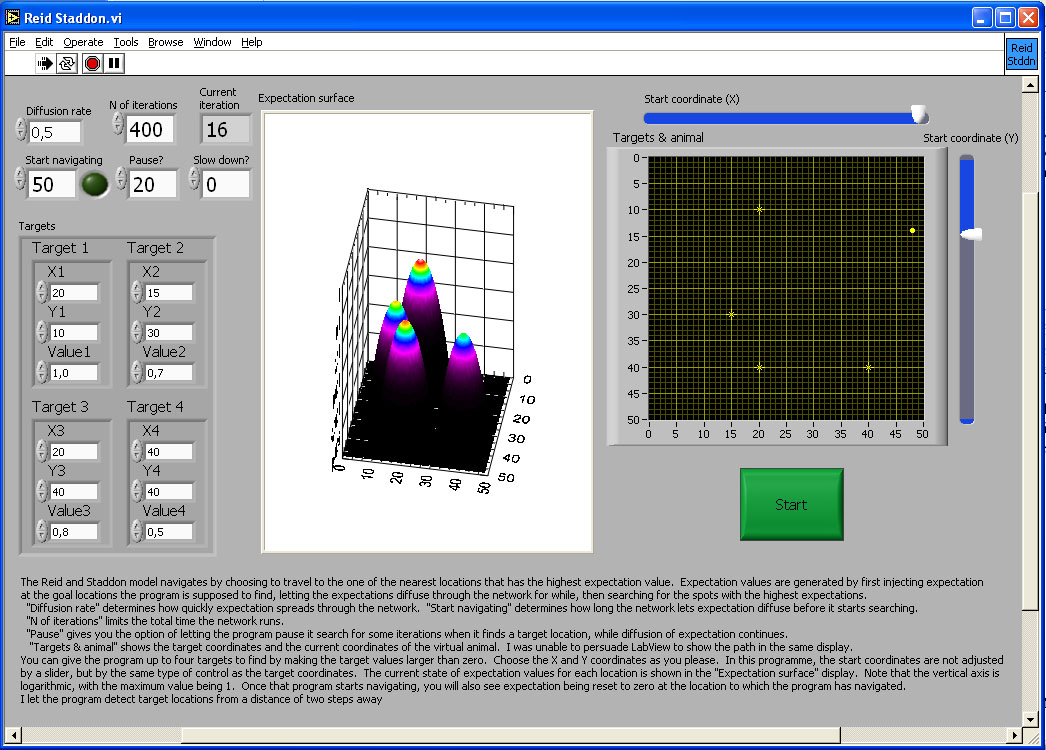
Reid and Staddon (1998) proposed a readout mechanism based on generalisation that does not explicitly deal with any spatial parameters at all. Instead, each location is attributed with an 'expectation' value. Initially only the goal locations have an expectation value above zero (see simulation, Figure 8). This expectation then spreads to neighbouring locations in a manner analogous to diffusion. The animal chooses a path by comparing, at each step, the locations immediately adjacent to its own and selecting the one with the highest expectation value. Whenever it fails to find reward or when it has consumed the reward it has found, it sets the expectation value at its current location to zero. This dynamic nature of the expectation surface prevents the animal from getting permanently caught in a local maximum of expectation. The computation of a path even between multiple goals is implicit in the generation of expectation values (see Bures, Buresova, & Nerad, 1992 and Cramer & Gallistel, 1997 for studies in rats and monkeys, respectively). The model copes with detours by cutting connections between appropriate expectation units, so that where there is an obstacle, there is also no diffusion of expectation. The expectation has to diffuse around this representation of the obstacle, setting a corresponding path in the real world.
Figure 8. Plots of expectation values for all locations in an area for Reid and Staddon’s (1998) model of the readout for a map. The simulation allows choice of up to four destination, with utility of the resources available at each destination ranging from 0 to 1. The model lets expectation diffuse through the network of expectation units for as many iterations, and with the diffusion parameter specified by the user. This simulation does not model obstacles. A model animal has started searching for reward from the specified starting point. At each point it chooses, it calculates a Gaussian weighted average of the expectation values of neighbouring units in order to choose the direction of the next step. If there is no reward, or when it has consumed reward, it sets expectation at its current location to zero, and decreases expectation in units corresponding to neighbouring locations according to a Gaussian weighting by distance. This pushes down the expectation surface and prevents the animal from backtracking immediately to an already depleted reward. As the animal moves away, expectation diffuses back in from neighbouring locations.
The image in the figure is a link to the simulation program. Click on the image to download or open the simulation program - in most operating system environments, you should be able to "open" the file to run the simulation without downloading it to your computer. However, you will probably FIRST have to download the LabView Runtime engine on your computer - and then INSTALL it - before being able to run this or the other simulations in this chapter.
Expectation at any one location thus depends on the initial expectation at a destination (i.e., the utility of the destination), the distance between destination and current location, how long and at what rate the expectation has been diffusing through the network, and the possible presence and shape of obstacles. The confounding of all these variables makes it impossible to select a goal based on resource or demand limits. An animal that only has enough time or energy to travel 1 km should not set out for a destination 5 km away, even if the rate of return is higher for the more distant destination. The same applies to an animal that has already eaten so much that it can eat only a little more.
IV. The Importance of Readout Mechanisms
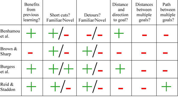
Four of the navigational systems discussed in this chapter do or can use the same representation of an animal’s own location, namely the hippocampal place field representation. Benhamou et al.’s (1995) mismatch minimisation algorithm uses the firing of place cells as retrieval cues for the snapshots taken at neighbouring locations, and then computes from the mismatches the best next step. Brown and Sharp (1995) proposed that place cell firing may serve to retrieve the responses in a map of stimulus-response associations. Burgess et al. (1994) use place cell firing to determine goal cell firing, which in turn serves to compute a vector to the destination. A neurophysiological version of the Reid and Staddon model (see Biegler, 2003) uses place cell firing to select the expectation units from which expectation should be read, to reset expectation, and to modulate the connections between expectation units and goal cells which provide the initial expectation. Although the representation of the animal’s location is identical, the four mechanisms that use this representation work according to different principles and give the resulting navigational systems radically different properties.
The mismatch minimisation model of Benhamou et al. depends on having stored snapshots, but does not need to store snapshots for specific purposes. Therefore it can benefit from exploration, taking novel paths over familiar areas. Learning in Brown and Sharp’s stimulus-response model is path-specific. On the way to a destination, an animal can use only the responses learned previously while underway to the same destination. No novel paths of any kind can be computed without new learning. The Burgess et al. readout mechanism benefits from previous experience in so far as it can use information about the locations of obstacles. The connections among Reid and Staddon’s expectation units are assumed to be established during exploration, and that information would still be useful when searching for a novel destination.
The mismatch minimisation model has no problems with familiar short cuts, as it can take any direct path to a destination over a familiar area. On unexplored area, it has no snapshots to retrieve, so it has no basis for choosing the next step. Brown and Sharp’s stimulus-response can create short cuts in so far as it can cut out loops, but cannot do anything where it has no associations to retrieve. Burgess et al.’s model can compute a vector at any place where its place fields and goal fields reach. The place fields may be completely or partly preconfigured, so exploration of an area is not essential. Short cuts over unfamiliar area are therefore possible. Reid and Staddon assumed that the connections among expectation units would only be set up with experience, precluding novel short cuts.
Benhamou et al.’s mismatch minimisation model has no mechanism for computing detours. Brown and Sharp’s stimulus-response model inevitably encodes detours made during exploration in its associations, but is restricted to find novel detours through trial and error; it has no way of computing a detour around a new obstacle. Burgess et al.’s goal cell model can detour around obstacles in locations already marked by goal cells, but also has nothing for computing a detour around a new obstacle. The same applies to the Reid and Staddon model: if there is a new obstacle, it would have to travel to the obstacle to interrupt the corresponding connections among expectation units before anything else could happen. Only Benhamou et al.’s model and Burgess et al.’s model can estimate the distance and direction to the goal, but none of the models is capable of estimating the distance between even just two remote points. Only the Reid and Staddon model can pick a path among multiple destinations by doing more than going to the nearest one.
Table 1: Summary of properties of four computational models.
It is also interesting to compare the models’ performances against those of animals. None of the models can identify landmarks on the basis of their spatial relationships to each other. Only the Burgess et al. model could actually extract the necessary information, if each landmark had a set of goal cells. The model would still need the same computational machinery to identify landmarks by their spatial relationships to each other as to solve the traveling salesman problem. The Reid and Staddon model’s solution to the traveling salesman problem does not involve computation of spatial relationships and so cannot be applied to the landmark identification problem. However, rats, pigeons and humans do fine on that problem (Cheng, 1986; Cheng & Gallistel, 1984; Cheng & Spetch, 1998; Hermer & Spelke, 1994, 1996; Kelly, Spetch, & Heth, 1998; Spetch, Cheng, & Macdonald, 1996; Spetch et al., 1997; see Pearce, Good, Jones, & McGregor, 2004, for results suggesting that rats use relationships between individual features, rather than computing global parameters).
Likewise, none of the models has any way of judging discrepancy between different sources of spatial information, and using that to weight accurate and reliable information. A variety of animals do so (Biegler & Morris, 1996, see discussion of directional cues; Cheng, 1988; Cheng, Collett, Pickhard, & Wehner, 1987; Chittka & Geiger, 1995a, 1995b; Etienne, Teroni, Hurni, & Portenier, 1990; Healy & Hurly, 1998; Kamil & Jones, 1997; Mackintosh, 1973; Rotenberg & Muller, 1997; see Bingman et al., this volume).
All the models require that an animal must be at a goal in order to register that location. They cannot specify a goal from a distance, an ability demonstrated by the observational learning seen in corvids or the path planning observed in toads (Bednekoff & Balda, 1996a, 1996b; Lock & Collett, 1979). An even more common and quite important problem for many animals is to determine whether a neighbour is encroaching on one’s territory. If the territory holder is to do that without going right up to the border (which may be enough to trigger a fight), the computational requirements are exactly the same: where is the possible intruder in relation to remote landmarks, and possible in relation to imaginary lines between landmarks? LaManna and Eason (2004) found that landmarks make the establishment of boundaries and sharing of space much easier and reduced border conflicts in blockheads. Eason, Cobbs, and Trinca (1999) reported that male cicada killer wasps even shifted territories so that the new boundaries coincided with landmarks that had been added specifically to lie within territories. The wasps benefited from less territorial conflict at boundaries marked by borders.
For much the same computational reasons, novel detours are a problem, but it is clear that at least some animals are less limited than the models: chameleons can detour around a gap without first trying to stretch across it, toads can detour around pits and fences, and jumping spiders can correctly choose a path that initially leads them away from and even out of sight of prey (Collett, 1982; Collett & Harkness, 1982; Jackson & Wilcox, 1993; Tarsitano & Jackson, 1997).
Spatial information is not only useful in finding foraging patches, but potentially also in deciding whether to leave a patch. The marginal value theorem (Charnov, 1976) only specifies that a forager should leave a patch when prey capture rate falls below the average for all foraging patches. Strictly speaking, that holds only for prey that moves randomly within the patch. If the prey is berries on a group of bushes, it would be good to know which bushes have already been picked. In other words, a foraging animal would benefit from a representation of areas already searched.
The Brown and Sharp model cannot do so. It is a reference memory system that only learns on arrival at a destination. What is needed instead is a temporary instruction to avoid areas already searched. The Burgess et al. model could, in principle, cope with that by temporarily changing the evaluation of what is at the places visited. But because the Burgess et al. model only considers goals one at a time, in order to decide whether to leave a patch it would be necessary to search the representation for all destinations within the patch, and check their status. The Reid and Staddon model has a temporary record of visited places already built in, in the form of the ‘inhibitory footprint’ that resets expectation to zero wherever the animal has just been.
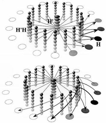
Figure 9. Computational map version of a continuous attractor model of head direction cells (Biegler, 1996; original frequency-coded version by Skaggs, Knierim, Kudrimoti, & McNaughton, 1995, cited in McNaughton et al., 1996). The H cells are head direction cells. Their shading represents activity level. The H’ cells code for turns, from a fast clockwise turn at the top of the column to a fast counterclockwise turn at the bottom, with intermediate speeds in between. In H’ and H’H cells, shading represents tuning to speed of turn. The H’H cells receive projections from both the H head direction cells and the H’ turn units, and fire only when there is simultaneous input from both sources. Each head direction cell is connected to all the H’H cells that code for the same direction, regardless of speed of turn. Each H’ unit is connected to all H’H units that code for the same speed of turning, regardless of head direction. The combination of speed of turn and head direction restricts activation to a small subset of H’H units.
The top diagram shows a slow counterclockwise turn. Straight lines show output from H’ and H cells to H’H units. Arrows represent the output from H’H cells to H cells, to update the estimate of head direction. Not shown are mutually inhibitory connections among H cells, which are weakest for cells with similar directional tuning and become stronger the more the characteristic directions of two cells differ. When cells at and beyond the counterclockwise border of the activity patch receive input, their inhibition of cells with substantially different directional tuning increases. That will decrease activity of cells at the clockwise end of the activity patch, which do not receive input from the H’H cells.
The lower diagram shows a fast clockwise turn. The turning speed of the activity patch is increased by the connections from H’H cells to H cells reaching further ahead of the activity patch. It would also be possible to use greater synaptic strength, either as an alternative or in addition. The original frequency-coded model can be thought of as a two-layer version of this model, for clockwise and counterclockwise turns, with the speed of turning represented by the firing frequency of H’ and H’H cells.
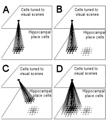
Figure 10. Resetting of path integration in the model of Samsonovich and McNaughton (1997) and removal of errors by averaging. For simplicity, place cells are arranged as if cells with adjacent place fields were also anatomically adjacent. Likewise a unit tuned to recognise a visual scene is shown as if units tuned to neighbouring scenes were anatomically adjacent. Place cells are represented by squares, whose size is proportional to the firing rate of the cell.
(A) Connections from a cell or group of cells tuned to a specific visual scene to simultaneously active place cells are potentiated. The more active a place cell is, the stronger the connection from the visual unit(s) to the place cell (shown here as the thickness of the connecting lines). In this example, visual unit(s) and place cells match up exactly.
(B) The animal finds itself at the point where it stored a visual scene, but due to an error in path integration the activity packet representing the animal's estimated position (grey squares on the lower right) is some distance from where it should be. Activation of the visual unit will excite the correct set of place cells through the connections established earlier. Inhibitory connections between place cells ensure that there can be only one stable activity packet in the place cell representation. When an activity packet is forced into existence at the coordinate to which visual units are linked (black squares), the original packet (grey squares) either moves there, or fades as a new one is created.
(C) If there was an error in path integration when the animal first linked a visual scene to place cells, and if the learning rate is high enough that learning effectively occurs in a single trial, any error made on that occasion will be retained. Recognition of the visual scene would reset path integration to the erroneous coordinates given when the animal established the link.
(D) If the learning rate is low enough that connections from the visual unit(s) to place cells are established over a number of visits to the resetting point, each with a randomly varying error in path integration, then connections from the visual unit(s) to place cells will cover a larger area, but are likely to be centred far more accurately on the correct coordinates. In Samsonovich and McNaughton's model, the broader spread of the connections would not affect the size of the activity packet, which is determined by inhibitory connections. Even if the activity packet established initially is large (as shown by the grey squares on the lower left of diagram D) it would shrink to normal size (black squares).In introducing the comparison of these four models I have been careful to claim only that they have an identical representation of the animal’s location, not of space. A representation of space properly must contain more than one point, yet the place cell representation shared by the four models does not, on its own, contain any information where anything else is or how to get there. That information is contained in, variously, stimulus-response associations, the snapshots loaded into the mismatch-minimization algorithm, goal cells and expectation surfaces. And although information storage thus differs between the models, I still argue that it is attention to readout that makes the differences clear. By the criterion that a representation of space must represent the spatial relationships between several points, the Brown and Sharp model does not even have a representation of space. Yet, when considering how information is used, the stimulus-response associations form a map. The Brown and Sharp model is just not able to read the whole map, it only ever looks at the animal’s current location. If outcomes are added to the responses, the animal can read from a very similar map of stimulus-(response-outcome) associations where each response will lead. It can look at the whole map.
It is necessary to emphasise how information is used, because the very natural and intuitive metaphor of the survey map is far too intuitive. It appears so obvious that the information in a survey map can be used to plan paths of all sorts that it detracts from the fact that the map itself does not do the path planning. That happens to automatically and unobtrusively in the human map reader’s mind that it tends to be forgotten (see Taylor & Rapp, this volume). But when trying to account for animals’ navigational abilities, it is crucial to find out how they use the information they acquired.
V. The Role of Path Integration
There is substantial disagreement over the role of path integration in navigation. Some authors argue it could be the basis of cognitive mapping (Gallistel, 1990; McNaughton et al., 1996; O’Keefe, 1976; Samsonovich & McNaughton, 1997; Touretzky & Redish, 1996; Wan, Pang, & Olton, 1994), others that it is a simpler alternative that must be ruled out when investigating short cut abilities (Bennett, 1996; Jacobs & Schenk, 2003). The difference appears to lie in how one thinks of path integration. It may be considered merely as providing a vector back to the most recent starting point (Jacobs & Schenk, 2003), which, of course, puts severe limits on its usefulness. However, that is far from being the only option.
Possible global path integration systems (as opposed to Collett et al.’s (1998) local vectors) may be reset only at the starting point or at other points as well, they may only be able to specify a vector back to the starting point, or to any arbitrarily chosen point, and there may be only one path integrator or several. The resulting eight combinations have been compared in detail elsewhere (Biegler, 2000). Here, I will examine only the single path integrator with multiple destinations and resetting points, because that is the simplest path integration system that will easily provide the kind of metric representation of space that is supposed to be characteristic of cognitive maps.
In neural network models of path integration, the representation of the animal’s location is generally assumed to be a continuous attractor, which means that the network has distinct stable states that can be changed continuously and in a predictable manner to represent locations and directions (Hartmann & Wehner, 1995; McNaughton et al., 1996; Samsonovich & McNaughton, 1997; Figure 9). A representation like the hippocampal place field representation can be generated by a continuous attractor network (Samsonovich & McNaughton, 1997). Then if the locations of two place fields in the environment are known, it is possible to predict the location of any other place field in the representation. (This argument ignores remapping, which is not relevant here; however, taking remapping into account only means that it is also necessary to identify which of several possible representations is currently active.) As a consequence of this predictability, once the path integration system has been anchored to some environmental features, it will have a preconfigured representation even for areas which the animal has not yet explored. A readout mechanism such as Burgess et al.’s goal cells can give an animal an estimate of distance and direction to any number of destinations at entirely arbitrary locations within the range of the representation.
Such a path integration system is therefore not limited to returning to a starting point. Because the network is preconfigured, the animal can take novel paths to a destination even across areas it has not explored. The ability to compute novel paths, especially novel short cuts (taking a novel path over unfamiliar area from a familiar starting position to a familiar destination) and instantaneous transfer (taking a novel path from an unfamiliar starting point to a familiar destination), is often considered the gold standard criterion for cognitive mapping. Fulfilling this criterion is trivially easy with such a path integration system, and path integration will necessarily provide a metric representation doing nothing more sophisticated with landmarks than recognizing them.
A possible objection to the idea of a navigation system being primarily based on path integration is that path integration is a recursive process, and therefore necessarily accumulates errors. An animal moves, estimates the movement it has made, updates its representation, and uses that updated representation complete with any error made in the estimation of the movement as the basis for the next update. Path integration therefore needs to be periodically reset by reference to external information. The system must have a way of determining what location its path integrator should represent at that moment, and update the representation if it deviates from where the animal really is. If that resetting required another landmark-based metric representation, one would argue that this landmark-based representation is primary, and path integration only a backup system, but that is not true. No metric representation outside a path integrator is needed for accurate resetting or for storage of accurate coordinates of destinations.
This claim depends on the following assumptions: 1) the representation of the animal’s location is distributed, as in the hippocampal place field representation; 2) learning rates are slow enough that learning is not complete in a single trial; and 3) errors are random, not systematic. (Footnote: The last assumption may be considered controversial, given that apparent systematic errors in return heading after an L-shaped outward journey have been reported in a variety of species, but the algorithm proposed by Müller and Wehner (1988) to account for these headings fails to account for hamsters’ headings after a loop in their outbound journey (Séguinot, Maurer, & Etienne, 1993). The apparent errors after L-shaped journeys may instead be a bias added on for the purpose of error correction, as they bring the animal near to landmarks recently seen on the outbound part of the journey.)
Given these assumptions, establishing an accurate coordinate for resetting or for a destination can be accomplished by connecting something as simple as a snapshot of landmarks to the then active units in the path integrator. On successive visits to the same spot, slightly different sets of units will be active, but if the representation in the path integrator is sufficiently distributed, these sets will overlap to form a single, larger set of units. As long as errors are random, this set of units connected to the representation of the snapshot will tend to settle on the correct coordinate. Resetting occurs when a view of the snapshot activates the connected units in the path integrator. Inhibition among units in the continuous attractor network will shrink the set of units down to normal size. This averaging process can, given enough sampling of a location, achieve any desired accuracy (Figure 10). Under the assumptions here, averaging is not merely simple, but inevitable (Biegler, 2000).
VI. Summary
A brief analysis of animals’ possible navigation strategies started with the basic problem "How can I get to a specific place X?," followed by an iterative procedure of finding a possible solution, exploring its limitations and using those limitations to define additional problems a navigational system may be required to solve. Very basic considerations served as the starting point. What is navigation good for? What is the minimum navigational capacity that is better than none at all, and what further additions to that minimum might be useful?
Six major conclusions can be drawn from the analysis above: 1.) The nature of the readout mechanism is as important as the kind of representation and the rules for storing information in it. The same representation of an animal’s location can be combined with very different readout mechanisms. The properties of the resulting combinations depend critically on the nature of the readout mechanism. 2.) Navigation is possible without representing spatial relationships. Many of the strategies discussed here do not use any information on angles, or distances between places, or even simpler geometric properties such as being between two points or being at the intersection of two lines. Instead, they specify procedures that take the animal closer to its destination. 3.) There is a whole spectrum of navigational systems, which do not fall into two distinct classes of simple associative models and complex mapping models. 4.) Readout mechanisms are often domain-specific and species-specific. Image matching is part of the bee’s navigational tool kit. But image matching will not tell the bee how much food to expect or when food is available. The image matching algorithm is domain-specific. Comparison with the navigational abilities of rodents and birds also indicates it is, if not species-specific, then at least taxon-specific (see Balda & Kamil, and Healy, this volume). 5.) The short cuts and instantaneous transfer often considered critical tests of cognitive mapping are computationally rather simple at the level of readout. The only question is whether the required information has been stored in the representation. Detours, spatial working memory (avoiding recently visited areas), identifying landmarks on the basis of their spatial relationships to each other, determining at a distance whether a neighbour has intruded into one’s own territory and judging the accuracy and reliability of spatial information; these not only appear to be computationally far more interesting problems, but animals have been shown to cope with these problems. Future modeling efforts should pay attention to such capacities. 6.) Path integration is sufficient to solve a wide range of ecologically relevant navigation problems, namely those that involve determining an animal’s own location relative to familiar other points, but does not help in establishing spatial relationships to a novel entity from a distance, for example, to determine whether another individual has intruded into one’s territory.
VII. References
Bednekoff, P.A. & Balda, R.P. (1996a). Social caching and observational spatial memory in pinyon jays. Behaviour, 133, 807-826.
Bednekoff, P.A., & Balda, R.P. (1996b). Observational spatial memory in Clark's nutcrackers and Mexican jays. Animal Behaviour, 52, 833-839.
Benhamou, S., & Bovet, P. (1992). Distinguishing between elementary orientation mechanisms by means of path analysis. Animal Behaviour, 43, 371-377.
Benhamou, S., Poucet, B., & Bovet, P. (1995). A model for place navigation in mammals. Journal of Theoretical Biology, 173, 163-178.
Biegler, R. (1996). Short and medium range navigation and its relationship to cognitive mapping and associative learning. Unpublished PhD thesis, University of Edinburgh, Edinburgh, Scotland.
Biegler, R. (2000). Possible uses of path integration in animal navigation. Animal Learning & Behavior, 28(3), 257-277.
Biegler, R. (2003). Reading cognitive and other maps: How to avoid getting buried in thought. In K. J. Jeffery (Ed.), The neurobiology of spatial behaviour. Oxford: Oxford University Press.
Biegler, R., & Morris, R.G.M. (1996). Landmark stability: Further studies pointing to a role in spatial learning. Quarterly Journal of Experimental Psychology, 49B(4), 307-345.
Blackford-Cook, S. (1969). Experiments on homing in the limpet Siphonaria normalis. Animal Behaviour, 17, 679-682.
Brown, M.A., & Sharp, P.E. (1995). Simulation of spatial learning in the Morris water maze by a neural network model of the hippocampus and nucleus accumbens. Hippocampus, 5(3), 171-188.
Brown, S.F., & Mellgren, R.L. (1994). Distinction between places and paths in rats' spatial representation. Journal of Experimental Psychology: Animal Behavior Processes, 20(1), 20-31.
Bures, J., Buresova, O., & Nerad, L. (1992). Can rats solve a simple version of the travelling salesman problem? Behavioural Brain Research, 52, 133-142.
Buresova, O., Homuta, L., Krekule, I., & Bures, J. (1988). Does non-directional signalization of target distance contribute to navigation in the Morris water maze? Behavioral and Neural Biology, 49(2), 240-248.
Burgess, N., Recce, M., & O'Keefe, J. (1994). A model of hippocampal function. Neural Networks, 7, 1065-1081.
Cartwright, B.A., & Collett, T.S. (1982). How honey bees use landmarks to guide their return to food. Nature, 295, 560-564.
Cartwright, B.A, & Collett, T.S. (1983). Landmark learning in bees: Experiments and models. Journal of Comparative Physiology, 151, 521-543.
Charnov, E.L. (1976). Optimal foraging: The marginal value theorem. Theoretical Population Biology, 9, 129-136.
Cheng, K. (1986). A purely geometric module in the rat's spatial representation. Cognition, 23, 149–177.
Cheng, K. (1988). Some psychophysics of the pigeon‘s use of landmarks. Journal of Comparative Physiology A. 162, 815-826.
Cheng, K. (1990). More psychophysics of the pigeon‘s use of landmarks. Journal of Comparative Physiology A. 166, 857-863.
Cheng, K. (2000). How honeybees find a place: Lessons from a simple mind. Animal Learning & Behavior, 28(1), 1-15.
Cheng, K., Collett, T.S., Pickhard, A., & Wehner, R. (1987). The use of visual landmarks by honeybees: Bees weight landmarks according to their distance from the goal. Journal of Comparative Physiology A, 161, 469-475.
Cheng, K., & Gallistel, C. R. (1984). Testing the geometric power of an animal's spatial representation. In H. L. Roitblat, T. G. Bever, & H. S. Terrace (Eds.), Animal cognition (pp. 409–423). Hillsdale, NJ: Erlbaum.
Cheng, K., & Spetch, M.L. (1998). Mechanisms of landmarks use in mammals and birds. In S. D. Healy (Ed.), Spatial representation in animals. Oxford: Oxford University Press.
Chew, G.L., Sutherland, R.J., & Whishaw, I.Q. (1989). Latent learning does not produce instantaneous transfer of place navigation: A rejoinder to Keith and McVety. Psychobiology, 17, 207-209.
Chittka, L., & Geiger, K. (1995a). The influences of landmarks on distance estimation of honey bees. Animal Behaviour, 50, 23-31.
Chittka, L., & Geiger, K. (1995b). Honeybee long-distance orientation in a controlled environment. Ethology, 99, 117-126.
Chittka, L., & Kunze, J. (1995). The significance of landmarks for path integration in homing honeybee foragers. Naturwissenschaften, 82, 341-343.
Clifford, K.T., Gross, L., Johnson, K., Martin, K. J., Shaheen, N., & Harrington, M.A. (2003). Slime-trail tracking in the predatory snail, Euglandina rosea. Behavioral Neuroscience, 117(5), 1086-1095.
Collett, M., & Collett, T.S. (2000). How do insects use path integration for their navigation? Biological Cybernetics, 83, 245-259.
Collett, M., Collett, T.S., Bisch, S., & Wehner, R. (1998). Local and global vectors in desert ant navigation. Nature, 394, 269-272.
Collett, T.S. (1982). Do toads plan routes? A study of detour behaviour in Bufo viridis. Journal of Comparative Physiology, 146, 261-271.
Collett, T.S. (1995). Making learning easy: The acquisition of visual information during the orientation flight of social wasps. Journal of Comparative Physiology A, 177, 737-747.
Collett, T.S. (1996). Insect navigation en route to the goal: Multiple strategies for the use of landmarks. Journal of Experimental Biology, 199(1), 227-235.
Collett, T.S., & Baron, J. (1994). Biological compasses and the coordinate frame of landmark memories in honeybees. Nature, 368, 137-140.
Collett, T.S., Dillmann, E., Giger, A., & Wehner, R. (1992). Visual landmarks and route following in desert ants. Journal of Comparative Physiology A, 170, 435-442.
Collett, T.S., & Harkness, L.I.K. (1982). Depth vision in animals. In D. J. Ingle, M. A. Goodale. & R. J. W. Mansfield (Eds.), Analysis of visual behavior. Cambridge, MA: MIT Press.
Cook, A. (1977). Mucus trail following by the slug Limax grossui Lupu. Animal Behaviour, 25, 774-781.
Cook, A., Bamford, O.S., Freeman, J.D.B., & Teidemann, D.J. (1969). A study of the homing habit of the limpet. Animal Behaviour, 17, 330-339.
Cramer, A.E., & Gallistel, C.R. (1997). Vervet monkeys as travelling salesmen. Nature, 387, 464.
Deutsch, J.A. (1960). The structural basis of behaviour. Cambridge: Cambridge University Press.
Eason. P.K., Cobbs, G.A., & Trinca, K.G. (1999). The use of landmarks to define territorial boundaries. Animal Behaviour, 58(1), 85-91.
Etienne, A.S., & Jeffery, K.J. (2004). Path integration in mammals. Hippocampus, 14(2), 180-192.
Etienne, A.S., Teroni, E., Hurni, C., & Portenier, V. (1990). The effect of a single light cue on homing behaviour of the golden hamster. Animal Behaviour, 39, 17-41.
Fitzgerald, T.D. (2003). Role of trail pheromone in foraging and processionary behaviour of pine processionary caterpillars. Thaumetopoea pityocampa. Journal of Chemical Ecology, 29(3), 513-532.
Frisch, K. von (1967). The dance language and orientation of bees. Cambridge, MA: Harvard University Press.
Gallistel, C.R. (1990). The organization of learning. Cambridge, MA: M.I.T. Press.
Gehlbach, F. R., Watkins, J. F., & Kroll, J. C. (1971). Pheromone trail-following studies of typhlopid, leptotyphlopid and colubrid snakes. Behaviour, 40, 282-294.
Gonor, J.J. (1967). Predator-prey reactions between two marine Prosobranch gastropods. The Veliger, 7, 228-232.
Hartmann, G., & Wehner, R. (1995). The ant's path integration system: A neural architecture. Biological Cybernetics, 73, 483–493.
Healy, S.D., & Hurly, T.A. (1998). Rufous hummingbirds' (Selasphorus rufus) memory for flowers: Patterns or actual spatial locations? Journal of Experimental Psychology: Animal Behavior Processes, 24, 396-404.
Hermer, L., & Spelke, E. (1994). A geometric process for spatial representation in young children. Nature, 370, 57-59.
Hermer, L., & Spelke, E. (1996). Modularity and development: The case of spatial reorientation. Cognition, 61, 195-232.
Jackson, D.E., Holcombe, M., & Ratnieks, F.L.W. (2004). Trail geometry gives polarity to ant foraging networks. Nature, 432, 907-909.
Jackson, R.R., & Wilcox, R.S. (1993). Observations in nature of detouring behaviour by Portia fimbriata, a web-invading agressive mimic jumping spider from Queensland. Journal of Zoology, London, 230, 135-139.
Kamil, A.C., & Jones, J.E. (1997). Clark's nutcrackers learn geometric relationships among landmarks. Nature, 390, 276‑279.
Keith, J.R., & McVety, K.M. (1988). Latent place learning in a novel environment and the influences of prior training in rats. Psychobiology, 16 (2), 146-151.
Kelly, D., Spetch, M.L., & Heth, C.D. (1998). Pigeon’s encoding of geometric and featural properties of a spatial environment. Journal of Comparative Psychology, 112, 259-269.
LaManna, J.R., & Eason, P.K. (2003). Effects of landmarks on territorial establishment. Animal Behaviour, 65, 471-478.
Lock, A., & Collett, T.S. (1979). A toad's devious approach to prey: A study of some complex uses of depth vision. Journal of Comparative Physiology, 131, 179-189.
Mackintosh, J.H. (1973). Factors affecting the recognition of territory boundaries by mice (Mus musculus). Animal Behaviour, 21, 464-470.
McNaughton, B.L., Barnes, C.A., Gerrard, J.L., Gothard, K., Jung, M.W., Knierim, J.J., Kudrimoti, H., Qin, Y., Skaggs, W.E., Suster, M., & Weaver, K.L. (1996). Deciphering the hippocampal polyglot: The hippocampus as a path integration system. Journal of Experimental Biology, 199, 173-185.
Mittelstaedt, H. (2000). Triple-loop model of path control by head direction and place cells. Biological Cybernetics, 83, 261-270.
Morris, R.G.M. (1981). Spatial localisation does not require the presence of local cues. Learning and Motivation, 12, 239-260.
Müller, M., & Wehner, R. (1988). Path integration in desert ants, Cataglyphis fortis. Proceedings of the National Academy of Sciences of the United States of America, 85, 5287-5290.
Muller, R.U., Stead. M., & Pach, J. (1996). The hippocampus as a cognitive graph. Journal of General Physiology, 107, 663-694.
O'Keefe, J. (1976). Place units in the hippocampus of the freely moving rat. Experimental Neurology, 51, 78-109.
O'Keefe, J., & Nadel, L. (1978). The hippocampus as a cognitive map. Oxford: Oxford University Press.
Paine, R. T. (1963). Food recognition and predation on Opisthobranchs by Navanax inermis. The Veliger, 6, 1-9.
Pearce, J.M., Good, M.A., Jones, P.M., & McGregor, A. (2004). Transfer of spatial behaviour between different environments: Implications for theories of spatial learning and for the role of the hippocampus in spatial learning. Journal of Experimental Psychology: Animal Behavior Processes, 30(2), 135-147.
Reid, A.K., & Staddon, J.E.R. (1998). A dynamic route finder for the congitive map. Psychological Review, 105, 585-601.
Rescorla, R.A. (1991). Associative relations in instrumental learning: The eighteenth Bartlett memorial lecture. Quarterly Journal of Experimental Psychology, 43B, 1-23.
Rotenberg, A., & Muller, R.U. (1997). Variable place-cell coupling to a continuously viewed stimulus: Evidence that the hippocampus acts as a perceptual system. Philosophical Transactions of the Royal Society of London B, 352, 1505-1513.
Samsonovich, A., & McNaughton, B. L. (1997). Path integration and cognitive mapping in a continuous attractor neuronal network model. Journal of Neuroscience, 17, 5900-5920.
Schölkopf, B., & Mallot, H.A. (1994). View-based cognitive mapping and path planning. Adaptive Behaviour, 3(3), 311-348.
Séguinot, V., Maurer, R., & Etienne, A.S. (1993). Dead reckoning in a small mammal: The evaluation of distance. Journal of Comparative Physiology A, 173, 103-113.
Skaggs, W.E., Knierim, J.J., Kudrimoti, H.S., & McNaughton, B.L. (1995). A model of the neural basis of the rat’s sense of direction. In G. Tesauro, D. Touretzky, & T. Leen (Eds.) Advances in neural information processing systems (Vol. 7). Cambridge, MA: MIT Press.
Spetch, M.L., Cheng, K., & Macdonald, S.E. (1996). Learning the configuration of a landmark array I: Touch-screen studies with pigeons and humans. Journal of Comparative Psychology, 110(1), 55-68.
Spetch, M.L., Cheng, K., Macdonald, S.E., Linkenhoker, B. E., Kelly, D. M., & Doerkson, S. R. (1997). Learning the configuration of a landmark array: II. Generality across search tasks. Journal of Comparative Psychology, 111(1), 14-24.
Steinhage, A., & Schöner, G. (1996). Self-calibration based on invariant view recognition: Dynamic approach to navigation. Robotics and Autonomous Systems, 20, 133-156.
Sutherland, R.J., Chew, G. L., Baker, J.C., & Linggard, R.C. (1987). Some limitations on the use of distal cues in place navigation by rats. Psychobiology, 15 (1), 48-57.
Tarsitano, M.S., & Jackson, R.R. (1997). Araneophagic jumping spiders discriminate between detours that do and do not lead to prey. Animal Behaviour, 53(2), 257-266.
Touretzky, D.S., & Redish, A.D. (1996). Theory of rodent navigation based on interacting representations of space. Hippocampus, 6, 247-270.
Wan, R.Q., Pang, K., & Olton, D.S. (1994). Hippocampal and amygdaloid involvement in nonspatial and spatial working memory in rats: Effects of delay and interference. Behavioral Neuroscience, 108, 866-882.
Webb, J.K., & Shine, R. (1992). To find an ant: Trail-following in Australian blindsnakes (Typhlopidae). Animal Behaviour, 43, 941-948.
Whishaw, I.Q. (1991). Latent leaning in a swimming pool place task by rats: Evidence for the use of associative and not cognitive mapping processes. Quarterly Journal of Experimental Psychology, 43B, 83-103.
©2006 All copyrights for the individual chapters are retained by the authors. All other material in this book is copyrighted by the editor, unless noted otherwise. If there has been an error with regards to unacknowledged copyrighted material, please contact the editor immediately so that this can be corrected. Permissions for using material in this book should be sent to the editor.